Exploratory Data Analysis and Visualization
Exploratory Data Analysis For Epidemiology
Learning objectives for this lesson:
- Explain the purpose of exploratory data analysis, how it differs from confirmatory analysis, and why summary statistics alone can mislead, using Anscombe's quartet as the illustration.
- Choose an appropriate display for one variable, for two variables and for many variables from the question and the types of the variables involved, and decide whether to show groups by colour or in separate panels (facets).
- Identify common poor displays (a truncated axis, bars of means without spread, a pie chart with many slices, overplotting, a dual axis, and colours that rely on telling red from green), describe what each conceals, and propose a better display.
- Read histograms and boxplots for shape, skew, outliers, ceilings, heaping, top-coding, impossible values and missing-value codes, and describe how to check, decide and report each problem and what it suggests for the later analysis.
- Explain in plain words what each part of the base R or ggplot2 code for a figure does (variables mapped to axes, colour or fill; boxes, jittered and see-through points, and smoothed lines with their confidence bands; facets, palettes, themes and saving with code), and describe what the resulting figure shows, including when a panel holds too few people to interpret.
- Interpret a correlation matrix, a correlation heatmap and a scatterplot with marginal histograms: describe a correlation by its direction and strength, explain when Spearman's correlation is preferred, and explain why a correlation cannot show a cause, a curved relationship or the shape of the data.
- Critique a combined multi-panel figure against the conventions of a publication figure, and write a caption that lets the figure stand on its own while leaving interpretation to the results text.
This course was developed by Dr. Kiffer G. Card based on Dohoo, I. R., Martin, S. W., & Stryhn, H. (2012). Methods in Epidemiologic Research. VER Inc.
Glossary: Key Terms, People & Concepts
📚 Reference page, available throughout the lesson
This glossary collects the key concepts, methods and people in this lesson. It can be used as a reference while working through the material or as a review before assessments. Typing in the search box filters the entries.
anscombe.
hist() in base R and geom_histogram() in ggplot2.
barplot(table(x)), and in ggplot2 with geom_bar() or geom_col().
pairs().
alpha in ggplot2 or rgb(..., alpha) in base R.
aes(), links a variable to a visual property such as horizontal position, colour or fill. A value given outside aes() is set for every mark.
geom_histogram(), geom_boxplot(), geom_point() or geom_tile(). Each geom is a layer.
facet_wrap() uses one variable, and facet_grid() places one variable in rows and another in columns.
theme_minimal().
geom_smooth(method = "loess").
cor().
ggExtra::ggMarginal() adds them to a ggplot2 scatterplot.
+ or | places plots side by side and / stacks them.
ggsave() writes a ggplot2 plot to a file of a chosen width and height. Resolution, in dots per inch (dpi), is usually 300 for print.
x[x == 20] <- NA. na.omit() keeps only rows with no missing values (a complete-case file).
Look Before You Model
The plots tell four different stories
anscombe.Four displays that conceal the data
Overview
Regression models for outcomes of many kinds rest on assumptions about the shape of the data: a straight-line relationship, residuals with an even spread, counts that are not more variable than the model allows, or observations that are independent. This lesson turns to the step that should come before any model is fitted, which is looking carefully at the data. Exploratory data analysis uses plots and simple summaries to find the shape of each variable, unusual or impossible values, and the relationships between variables. It tells the analyst whether the planned model suits the data, and it often suggests questions that the model should answer. This section explains what exploration is and how it differs from confirmatory analysis, uses Anscombe's quartet to show why summary statistics alone can mislead and reproduces the quartet in R, sets out how the number and the type of the variables in a question point to a display and when groups are better shown by colour or in separate panels, and ends with a gallery of common displays that conceal more than they reveal.
Learning Objectives
- 1.1 Explain the purpose of exploratory data analysis and how it differs from confirmatory analysis.
- 1.2 Use Anscombe's quartet to explain why summary statistics alone can mislead.
- 1.3 Compute summary statistics and draw a set of four plots in R for Anscombe's quartet, and say what the plots show that the statistics do not.
- 2.1 Choose an appropriate display for one variable, for two variables and for many variables, given the variable types involved.
- 2.2 Decide whether groups are better shown by colour within one panel or in separate panels (facets).
- 3.1 Recognize common poor displays (a truncated axis, means without spread, a pie chart with many slices, overplotting and a dual axis), describe what each one conceals, and name a better display.
1.1 What Exploratory Data Analysis Is
Exploration is easiest to understand when it serves a concrete request. The case below introduces the request that runs through the whole lesson, a one-page visual briefing on social connection that an analyst prepares for a regional working group on loneliness, and it names the survey from which every plot is drawn.
A regional health authority has formed a working group on loneliness. Before it commissions any statistical modelling, the group has asked an analyst for a one-page visual briefing on social connection, drawn from the 2021 wave of the Canadian Social Connection Survey (CSCS). The group has three questions: how lonely people in the survey are, whether loneliness differs by age and gender, and how loneliness goes together with social support and mental health. The 2021 wave has 4,045 respondents, one row per person, and 3,083 of them answered every question used in the briefing. Each section of this lesson adds plots to the briefing, and Section 4 assembles them into a single multi-panel figure with a caption. Section 2 describes how the survey recruited its respondents and what its sample can support.
Before drawing anything for the working group, the analyst needs to be clear about what kind of work the briefing is. The statistician John Tukey set out this kind of work in his book Exploratory Data Analysis (Tukey, 1977). He distinguished two activities. Confirmatory analysis tests a question that was set before the data were examined, and it reports estimates, confidence intervals and p-values. Exploratory analysis asks what the data look like, using plots and simple summaries, and it is open to finding things that nobody planned to look for. Tukey compared exploration to detective work: the analyst gathers clues about the data before deciding which formal test or model to apply.
Exploration serves three purposes in an epidemiological analysis. The first is to check data quality. By this we mean looking for values that are impossible (such as an age of 250), implausible (such as a person who reports working more than 16 hours a day, every day) or suspiciously common (such as an unexpected crowd of people at the top of a scale). Values like these usually point to a recording error, a coding rule or a problem with the question, and they need to be resolved before any result can be trusted. The second purpose is to describe distributions, that is, how the values of each variable are spread out. The shape of a distribution decides how the variable should be summarized and used. For example, a mean is a fair summary of a roughly symmetric variable, whereas a median is better for a skewed one, because a few very large values pull the mean toward them. A strongly skewed or oddly shaped variable may also need to be transformed or grouped before it enters a model. The third purpose is to show relationships between variables. Here the analyst asks whether two variables rise together or move in opposite directions, whether the relationship follows a straight line or a curve, and whether it looks different in different groups, such as women and men. The answers decide how each variable should enter a model, for example as a straight-line term, as a curve or in groups. This lesson develops the basic plots for one and two variables (histograms, boxplots, bar charts and scatterplots) into an exploratory workflow and adds displays for many variables.
Table 6.1 sets out five questions that the analyst asks during exploration, what a plot can show in answer to each, and how the answer changes the later analysis.
Table 6.1. Questions asked during exploration, what a plot can show, and what the answer changes in the analysis.
| Question the analyst asks | What the plot can show | What it changes in the analysis |
|---|---|---|
| What shape does each variable have? | Symmetry or skew, one peak or two, a floor or ceiling | The choice between a mean and a median; transformation or grouping |
| Are there unusual or impossible values? | Outliers, values outside the possible range, spikes at a maximum | Checking the codebook; recoding values to missing; a sensitivity analysis |
| Do answers pile up on particular values? | Heaping on round numbers or on the end of a scale | Caution in interpreting small differences; grouping the variable |
| How do two variables go together? | Direction, form (straight or curved) and strength | How each variable enters a model; whether a curve is needed |
| Does a pattern differ between groups? | Different shapes or slopes in different panels | Whether an interaction or a stratified analysis is needed |
Each question in Table 6.1 is answered by looking at a plot rather than by reading a single number. The next subsection shows, with four small datasets, why a summary statistic cannot take the place of that look.
1.2 Why Summary Statistics Alone Can Mislead
In 1973 the statistician Francis Anscombe published four small datasets to argue that graphs are an essential part of statistical analysis and that a computer should produce graphs as well as calculations (Anscombe, 1973). Each dataset has eleven pairs of values, labelled x and y, and the four datasets are supplied with R as a data frame called anscombe. Their summary statistics are almost identical, as Table 6.2 shows.
Table 6.2. Summary statistics for the four datasets in Anscombe's quartet (Anscombe, 1973).
| Statistic | Set 1 | Set 2 | Set 3 | Set 4 |
|---|---|---|---|---|
| Mean of x | 9.0 | 9.0 | 9.0 | 9.0 |
| Mean of y | 7.5 | 7.5 | 7.5 | 7.5 |
| Standard deviation of x | 3.32 | 3.32 | 3.32 | 3.32 |
| Standard deviation of y | 2.03 | 2.03 | 2.03 | 2.03 |
| Correlation of x and y | 0.816 | 0.816 | 0.816 | 0.817 |
| Fitted line | y = 3.00 + 0.500x | y = 3.00 + 0.500x | y = 3.00 + 0.500x | y = 3.00 + 0.500x |
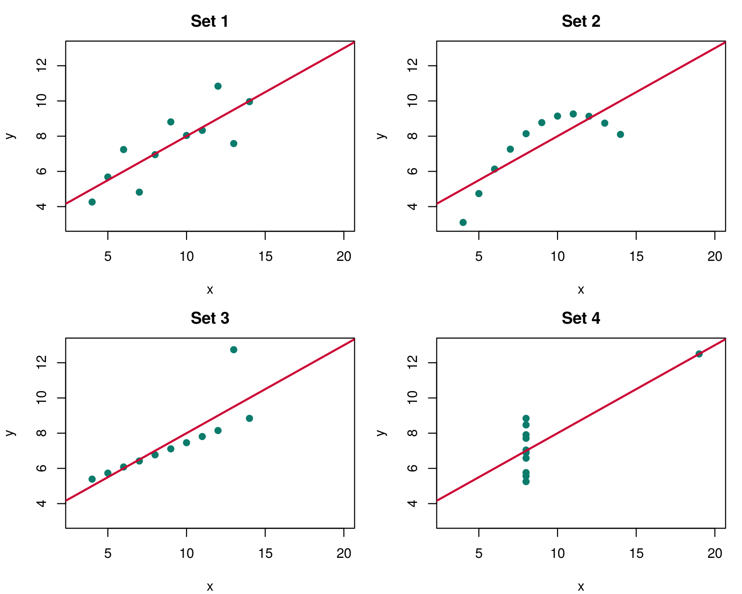
A report that gave only these numbers would describe the four datasets as the same. The plots show that they are very different. Figure 6.1 draws each of the four sets as a scatterplot with its fitted line.
anscombe data frame in R.Each set in Figure 6.1 fails or passes for a different reason, and the reasons are the ones an analyst meets in real data. Expand each panel of the accordion below to read what the plot of that set shows and whether the fitted line is a fair summary of it.
The points scatter evenly around a straight line. A correlation of 0.82 and a fitted slope of 0.5 are fair summaries of these data, and the assumptions of linear regression look reasonable.
The points follow a smooth arch with almost no scatter. The relationship is strong, but it is curved, so a straight line misdescribes it: the line overestimates y at both ends and underestimates it in the middle. A model with a squared term for x would fit these data almost exactly.
Ten points lie almost exactly on a line, and one point lies far above it. That single point pulls the fitted line upward and lowers the correlation from nearly 1 to 0.82. The analyst would check whether the point is a recording error before deciding how to handle it.
Ten of the eleven points share the same value of x (8), so within those points there is no relationship to estimate. A line describes how y changes as x changes, and among points that all have the same x there is no change in x from which to learn this. The one point at x = 19 therefore creates the whole correlation and decides the slope of the line on its own: if that point were moved up or down, the line would swing to follow it. In regression terms, the point has the highest leverage possible, so much influence that the fitted line passes exactly through it (R cannot even calculate a Cook's distance for such a point). Leverage describes how far a point lies from the other points along the x axis. By this we mean that a point with an unusual value of x has more power to tilt the fitted line than a point near the middle of the data, in the way that a long lever moves a load more easily than a short one. Cook's distance describes how much the fitted line would change if the point were removed. Here the point lies so far from the others along the x axis that the fitted line must pass through it, and without it the data would contain no information about the slope at all.
Taken together, the four panels show one fair summary, one wrong shape, one outlier and one influential point, all hidden behind the same numbers. The same lesson has been repeated with more recent examples. Starting from a dataset drawn in the outline of a dinosaur by Alberto Cairo, Matejka and Fitzmaurice (2017) generated the "Datasaurus Dozen", a set of further datasets that form stars, circles and lines, each with the same means, standard deviations and correlation as the dinosaur to two decimal places. The point is the same as Anscombe's: a summary statistic describes one feature of the data, and only a plot shows whether that feature is the one that matters. Because the quartet is supplied with R, this claim can be checked directly, which the next subsection does.
1.3 Anscombe's Quartet in R
Activity 6.1 reproduces Table 6.2 and Figure 6.1 from the anscombe data frame. It prints the means and standard deviations with colMeans() and sapply(anscombe, sd), the four correlations with cor() and the intercept and slope of each fitted line with coef(lm(...)), and it then draws the four scatterplots in one window with par(mfrow = c(2, 2)), adding the line y = 3 + 0.5x to each with abline(). Download the code and run it along with the text version below. As you run it, compare the console output for the four sets, which is almost identical, with the four plots, which are not; the questions then ask what an analyst who saw only the numbers would conclude, what each plot shows, and what to do about the single point that pulls set 3 away from its line.
Text version of the activity: the code of the run-along script, its console output and notes on reading it.
anscombe                          # four small datasets that come with R
round(colMeans(anscombe), 2)      # the mean of each column
round(sapply(anscombe, sd), 2) # the standard deviation of each columnThe data frame has eleven rows and eight columns: x1 and y1 form set 1, x2 and y2 form set 2, and so on. colMeans() gives the mean of every column, and sapply(anscombe, sd) applies the standard deviation function sd() to every column. Every x column has a mean of 9.0 and a standard deviation of 3.32, and every y column has a mean of 7.5 and a standard deviation of 2.03. In row 3, set 3 has y = 12.74, well above its neighbours.
round(cor(anscombe$x1, anscombe$y1), 3)   # correlation in set 1
round(cor(anscombe$x2, anscombe$y2), 3)   # set 2
round(cor(anscombe$x3, anscombe$y3), 3)   # set 3
round(cor(anscombe$x4, anscombe$y4), 3)   # set 4
coef(lm(y1 ~ x1, data = anscombe))        # intercept and slope, set 1
coef(lm(y3 ~ x3, data = anscombe))        # set 3
coef(lm(y4 ~ x4, data = anscombe)) # set 4The four correlations are 0.816, 0.816, 0.816 and 0.817. lm(y1 ~ x1, data = anscombe) fits a straight line, and coef() prints its intercept and slope: about 3.00 and 0.500 in sets 1, 3 and 4 (set 2 gives the same line).
par(mfrow = c(2, 2))    # four plots in one window: two rows, two columns
plot(anscombe$x1, anscombe$y1, main = "Set 1", xlab = "x", ylab = "y")
abline(3, 0.5, col = "red")       # add the line y = 3 + 0.5x
plot(anscombe$x2, anscombe$y2, main = "Set 2", xlab = "x", ylab = "y")
abline(3, 0.5, col = "red")
plot(anscombe$x3, anscombe$y3, main = "Set 3", xlab = "x", ylab = "y")
abline(3, 0.5, col = "red")
plot(anscombe$x4, anscombe$y4, main = "Set 4", xlab = "x", ylab = "y")
abline(3, 0.5, col = "red")
par(mfrow = c(1, 1))    # back to one plot per window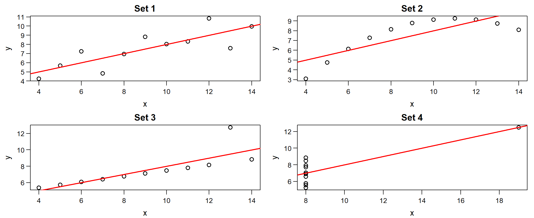
These lines print nothing to the console. They draw four scatterplots in the Plots pane, arranged in two rows and two columns by par(mfrow = c(2, 2)), and abline(3, 0.5, col = "red") adds the line y = 3 + 0.5x to each one, as in Figure 6.1. Section 2 explains par(mfrow = ...) in more detail.
R Reflect on what you just ran
Answer each question from your own output, as on the final exam: read the numbers, describe what the plots show, and decide what to do about an unusual point.
1. Using your console output, list the statistics that the four sets share. Interpret the correlation of 0.816 in one sentence. What would an analyst who saw only these numbers conclude about the four sets?
2. Describe the pattern in each of your four plots. For which set is the line y = 3 + 0.5x a fair summary? What do the plots show that the correlation of 0.816 does not?
3. Run your own code: at the end of the script, type coef(lm(y3 ~ x3, data = anscombe[-3, ])) and cor(anscombe$x3[-3], anscombe$y3[-3]) and run them. They refit set 3 without row 3, the point far above the line. What does that one point do to the slope and the correlation? Should it be removed from the analysis, and what would you do next?
Your output and plots make the point of the quartet concrete: the statistics agree to two decimal places, and only the plots show that the line y = 3 + 0.5x suits set 1 alone. Since a plot is needed before any summary can be trusted, the analyst must next decide which plot to draw for each question.
2.1 Matching the Display to the Question
Choosing a display begins with two questions about the request: how many variables it involves, and what type each variable is. Variables fall into two broad types. A numeric variable records an amount and is continuous (any value in a range, such as age) or discrete (whole numbers, such as the number of people in a household). A categorical variable places each person into a group and is binary, ordinal (ordered groups, such as self-rated mental health from poor to excellent) or nominal (unordered groups, such as province). Scale scores such as the loneliness score, which takes the whole-number values 3 to 9, are numeric for plotting purposes, although their small number of distinct values affects how they look, as later sections show.
Lesson 2 already matched the basic plots to these two questions. The recall below restates that guide, and its retrieval question asks you to apply it to the working group's question about age before you read on.
Recall: Lesson 2, Section 3 (Visualization Techniques)
Lesson 2, Section 3 matched the basic plots to the question and the variable type. A histogram shows the distribution of one numeric variable, a bar chart shows the frequencies of a categorical variable, boxplots compare a numeric variable across groups, and a scatterplot shows the relationship between two numeric variables. This section extends that guide to pairs of categorical variables and to many variables at once.
Retrieval question. Which display would you draw to see whether loneliness scores differ between four age groups, and why?
Figure 6.2 extends that guide into a decision tree, which starts from the number of variables in the question and then branches on their types.
A histogram divides the range of a numeric variable into intervals (bins) and draws a bar for the number of people in each one, so the bars touch and their order follows the number line. A bar chart draws one bar for each category of a categorical variable, with gaps between the bars, and the categories can be placed in any sensible order, such as the order of an ordinal scale or from most to least common. Students often confuse the two because both use bars. The test is the variable on the horizontal axis: a histogram has a numeric axis, and a bar chart has categories.
For two variables, the display follows the pair of types. A scatterplot places one point per person for two numeric variables. Boxplots side by side compare a numeric variable across the groups of a categorical variable, and adding the individual points shows how many people are in each group and how their values are spread. For two categorical variables, a bar chart of percentages (for example, the percentage of each gender in each mental health category) compares the groups fairly when the groups differ in size. By this we mean that each bar shows the share of a group that gave an answer, rather than the number of people who gave it. This matters because raw counts mix two things together: the size of the group and the pattern of answers within it. For example, there are far fewer non-binary respondents than women or men in the briefing file, so in a bar chart of counts every bar for non-binary respondents would be short, even if they rated their mental health in much the same way as everyone else. Converting the counts to percentages within each gender removes the difference in group size, so the bars answer the question that was actually asked, which is whether the pattern of ratings differs between the groups. For many variables, a scatterplot matrix or a correlation heatmap gives an overview of every pair, and facets repeat one display for each group in a grid of small panels, an idea that Tufte (1983) called small multiples.
Interactive 6.1 lets you practise the decision tree in Figure 6.2 on six requests from the working group. For each request, name the number and the type of the variables first, then click the display you would draw; the feedback under the options explains why each choice suits the request or fails it, and nothing is scored.
📊 Interactive 6.1: Try it: choose a display for the briefing
Each request below comes from the working group. Choose the display you would draw first. Feedback appears under the options, and nothing is scored.
1. How are loneliness scores (a numeric score from 3 to 9) distributed across the 3,083 people in the briefing file?
2. How many people rated their mental health as poor, fair, good, very good or excellent?
3. Does loneliness (numeric) differ between the four age groups (categorical)?
4. Is higher social support (a numeric score from 1 to 7) associated with lower loneliness?
5. Do women, men and non-binary respondents differ in how they rate their mental health (both categorical)?
6. Which of six numeric briefing variables (loneliness, support, depression, anxiety, life satisfaction and age) go together?
Several of the requests in Interactive 6.1 compare groups, such as genders or age groups. Once the type of display is settled, such a request raises one more choice, which is how the groups are told apart.
2.2 Colour or Separate Panels for Groups
Many questions in the briefing compare groups: women, men and non-binary respondents, or four age groups. Whatever display is chosen, the groups can be told apart by colour within one panel, or the display can be drawn once per group in panels that share a scale, which are called facets, or small multiples. Which works better depends on how many groups there are, how much their values overlap and how different their sizes are, as the rule below sets out.
Colour or facets?
When a display must show groups, the analyst can give each group its own colour within one panel, or draw one panel per group (facets). Colour works well for two or three groups whose values overlap little, and it lets the reader compare the groups directly. Facets work better when there are more groups, when the points overlap heavily, or when the groups differ greatly in size, because each group gets its own space on a shared scale.
The briefing uses both. In Section 3, three genders are told apart by fill colour within each age group (Figure 6.18), because three groups of boxes side by side are easy to compare, whereas twelve combinations of gender and age group each get their own panel (Figure 6.17), because twelve overlapping clouds of points could not be separated by colour and the small non-binary groups would be hidden behind the large ones. Whether groups are shown by colour or by panel, a display of the right type can still mislead when it is drawn poorly, and the last subsection examines the most common faults.
3.1 Common Poor Displays and What They Conceal
3.1.1 Four Displays That Conceal the Data
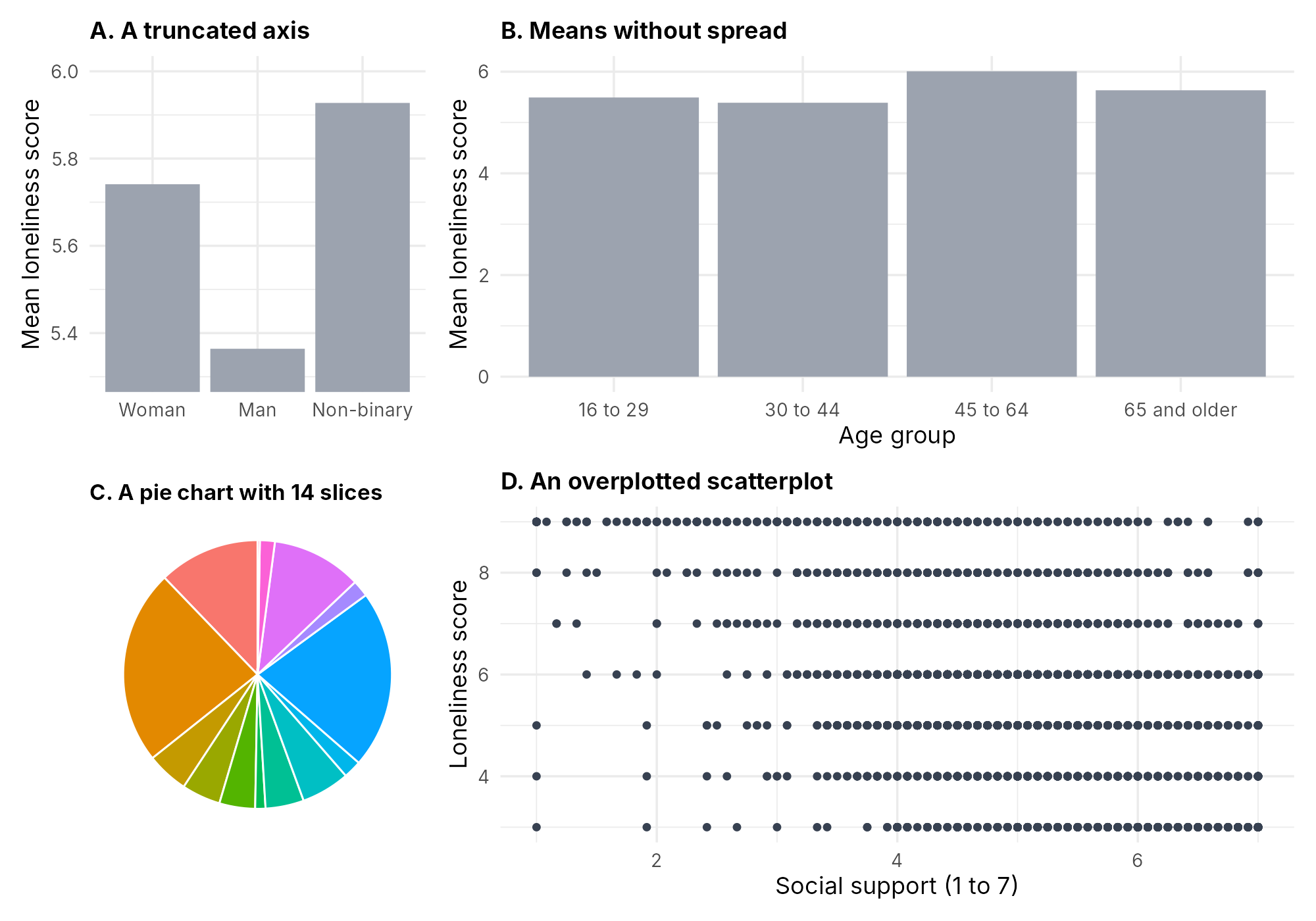
Research on graphical perception, the study of how accurately people read values from a graph, has found that people judge positions along a common scale more accurately than lengths, angles or areas (Cleveland & McGill, 1984). By this we mean that a reader can tell quite precisely which of two points placed against the same axis is higher, but is much less precise when asked which of two pie slices is larger or how much bigger one circle is than another. This finding gives a practical rule for building displays. A good display encodes the comparison that matters as a position or a length on a shared axis, so that the reader makes the comparison with the least error. In addition, a good display shows the data themselves wherever possible rather than a single summary of them, because, as Anscombe's quartet showed, a summary can hide the very shape that matters. Four displays that break these principles are common in reports and presentations: a bar chart whose axis does not start at zero, bars of group means that hide the spread, a pie chart with many slices, and a scatterplot in which the points cover one another. Each was drawn from the briefing file, beside a better version.
The four tabs below hold Figure 6.3 (a truncated axis), Figure 6.4 (means without spread), Figure 6.5 (a pie chart with many slices) and Figure 6.6 (overplotting). Open each tab, compare the poor version on the left with the better one on the right, and read under each figure what the poor version conceals; the first tab also explains the dual axis, a related distortion.
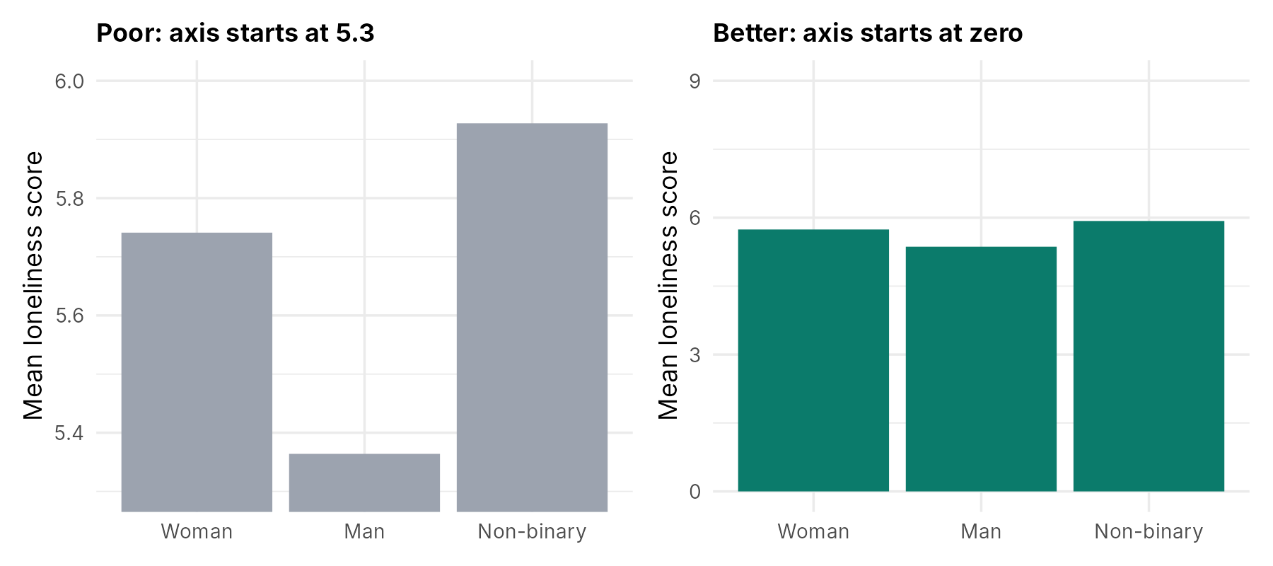
What it conceals. A bar encodes a value by its length, so a bar chart whose axis starts above zero misrepresents every comparison. On the left, the bar for men looks about one tenth of the height of the bar for non-binary respondents, although the means are 5.36 and 5.93, a ratio of about nine to ten. The right panel starts the axis at zero, so the lengths are proportional to the values. A related distortion is the dual axis, in which two series share a plot with two different vertical scales, one on the left and one on the right. Because the analyst chooses each scale separately, either series can be stretched or squeezed at will. For example, by changing the range of the right-hand axis, the same two series can be made to look as if they rise together, cross at a dramatic point, or barely move relative to each other. The apparent crossing points and relative heights therefore depend entirely on how the two scales were chosen rather than on the data, and two separate panels, each with its own clearly labelled axis, are usually clearer.
Note on axis ranges. The zero rule applies to bars. A dot or line display may use an axis that covers the possible range of the scale (3 to 9 for this loneliness score), provided the range is labelled.
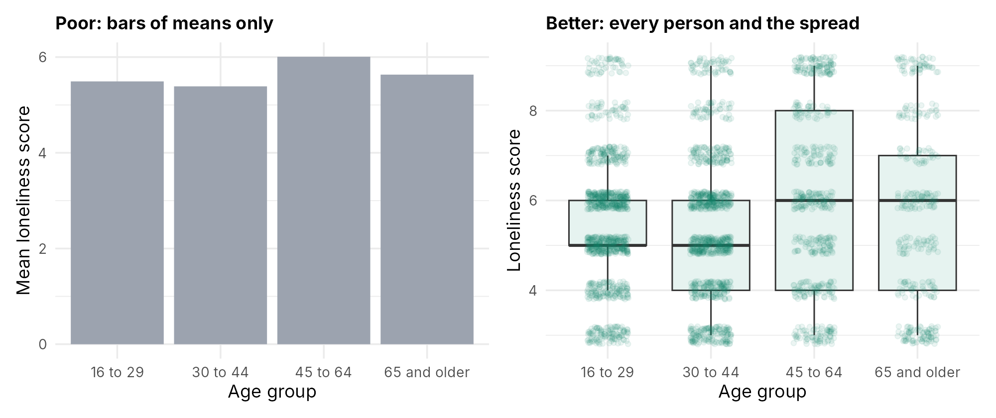
What it conceals. The bars show four means between 5.39 and 6.01 and nothing else. They hide the spread within each group (scores from 3 to 9 in every group), the shape of each distribution, and the number of people in each group, which ranges from 366 people aged 65 and older to 1,079 people aged 16 to 29. Weissgerber and colleagues (2015) reviewed 703 research articles in leading physiology journals, found that bar graphs were the most common way of presenting continuous data (85.6% of the articles included at least one), and recommended displays that show the distribution of the data, particularly dot plots of the individual values when samples are small. The right panel shows that the differences between age groups are small compared with the variation within each group.
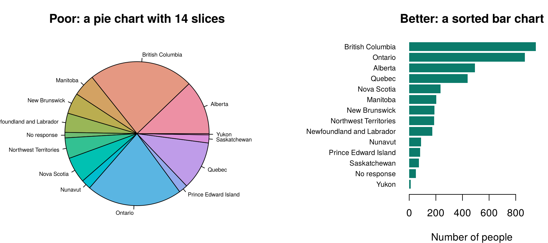
What it conceals. A pie chart asks the reader to compare angles and areas, which people judge less accurately than positions along a common scale. With fourteen slices, several of them thin, it is hard to tell whether Manitoba or New Brunswick has more respondents, or to read the smaller territories at all. The sorted bar chart places every category on a common scale, so the order and the size of the differences are clear. A pie chart can be acceptable for two or three categories that make up a whole; for more categories, a bar chart is clearer.
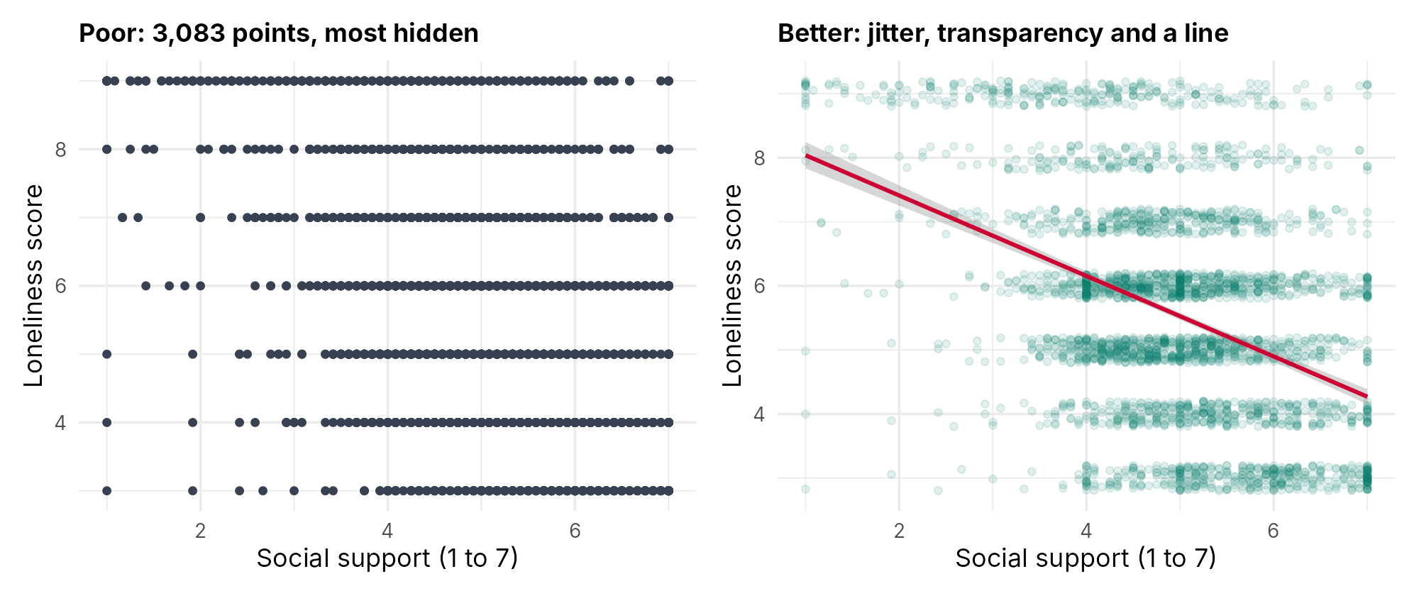
What it conceals. The loneliness score takes only seven values, so 3,083 points fall on seven horizontal lines and lie on top of one another. The left panel cannot show where most people are, and a row with five people looks the same as a row with five hundred. The right panel adds a small random vertical shift to each point (jitter) and draws the points with transparency, so dense areas look darker. The fitted line makes the downward trend easy to see: people with more social support tend to report less loneliness.
In each tab, the poor display hides either the comparison that matters or the data themselves, and the better version puts the comparison on a common scale and shows the people behind it.
3.1.2 Smaller Faults in Draft Figures
The four tabs show displays of the wrong form. Draft figures also fail in three smaller ways, and a critique of a figure should look for these as well. The first is labelling: an axis titled with an R variable name (such as life_sat) or a single letter (such as "y"), or with no units, leaves the reader to guess what is shown, so each axis is labelled in words with its units or range. The second is colour that carries no information or that relies on telling red from green: bright fills that only repeat the labels on the axis add nothing, and about 8% of men of northern European ancestry cannot tell red from green, so one plain colour, or a colour-blind-safe palette (Section 3), is the fix. The third is missing context: no sample size, data source or period anywhere in the figure, which the caption supplies (Section 4). When you critique a figure, state each problem, say what a reader could get wrong because of it, and give the fix.
This section has explained why the analyst looks at the data before fitting a model, how the question and the variable types point to a display and how groups are best shown, and what common poor displays conceal. The key takeaways below gather these ideas, the knowledge check reviews them, and Section 2 draws the displays for the briefing file in base R.
Key Takeaways
- 1.1 Exploratory data analysis is the step where you look carefully at the data before fitting any model. Using plots and simple summaries, you find the shape of each variable, any unusual or impossible values, and how the variables go together. Confirmatory analysis is different: it tests a question that was set before the data were examined, and it reports estimates, confidence intervals and p-values. Exploration comes first because it tells you whether the planned model suits the data, and Table 6.1 links what each plot can show to what it changes in the analysis. When a question asks you to classify an activity, ask whether the question was fixed in advance and answered with a formal estimate or test (confirmatory), or whether the analyst is looking to see what the data contain, for example by checking for impossible values (exploratory).
- 1.2 Anscombe's quartet is the classic warning that summary statistics can hide very different data. Its four small datasets share almost the same means, standard deviations, correlation (about 0.82) and fitted line (y = 3.00 + 0.500x), yet one follows a straight line, one is a smooth curve, one is a near-perfect line pulled away by a single outlier, and in one a single point creates the whole relationship. A summary statistic describes one feature of the data, and only a plot shows whether that feature is the one that matters. So if a question gives you only a correlation or a fitted line and asks what you can conclude, the safe answer is that you cannot tell whether the line is a fair summary until you have seen a scatterplot, because a curve, an outlier or one influential point could give the same numbers.
- 1.3 Activity 6.1 lets you see this for yourself in R.
colMeans(anscombe),sapply(anscombe, sd),cor()andcoef(lm(y1 ~ x1, data = anscombe))give almost identical numbers for all four sets, while the four scatterplots drawn afterpar(mfrow = c(2, 2))look completely different. The fitted line is a fair summary only for set 1: set 2 is curved, in set 3 one outlier distorts the slope, and in set 4 one point at x = 19 decides the line on its own. When you describe output like this, first list what the sets share, then say in one sentence what each plot shows, and finish by saying which summary the plots support and which they do not. - 2.1 Choosing a display starts with two questions: how many variables the question involves, and what type each one is (numeric or categorical). For one numeric variable, draw a histogram; for one categorical variable, draw a bar chart of counts, keeping ordered categories in their scale order. For two numeric variables, use a scatterplot; for a numeric variable across groups, use boxplots with the individual points; and for two categorical variables, use a bar chart of percentages within each group, so that groups of different sizes are compared fairly. For many numeric variables, a correlation heatmap or a scatterplot matrix gives an overview of every pair. A common trap is confusing a histogram with a bar chart because both use bars: check the horizontal axis, which is a number line for a histogram and a set of categories for a bar chart. On an exam, name the variable types first and let them lead you to the display, as the decision tree in Figure 6.2 does.
- 2.2 When a display has to show groups, you can give each group its own colour within one panel, or draw a separate panel for each group (facets, also called small multiples). Colour works well for two or three groups whose values overlap little, because the reader can compare them directly on the same axes. Facets work better when there are many groups, when the points overlap heavily, or when the groups differ greatly in size, because each group then gets its own space on a shared scale and a small group is not hidden behind a large one. When a question describes the groups, count them and ask how much they overlap and how different their sizes are. In this lesson, for example, three genders are told apart by fill colour within each age group (Figure 6.18), while twelve combinations of gender and age group each get their own panel (Figure 6.17).
- 3.1 A display of the right type can still mislead when it is drawn poorly, and each common fault hides something specific. A bar chart whose axis starts above zero exaggerates differences, because readers judge a bar by its length, so the axis of a bar chart starts at zero. Bars of group means hide the spread, the shape and the number of people in each group, and boxplots with the individual points show all three. A pie chart with many slices asks readers to compare angles, which they do poorly, so a bar chart sorted by count is clearer; overplotting hides where most people are, which jitter and transparency fix; and a dual axis makes any crossing depend on how the two scales were chosen, so two separate panels are clearer. Check the smaller faults too: axes titled with R names such as
life_sator a single letter, colour that only repeats the labels or relies on telling red from green, and no sample size or data source. When you critique a figure, state each problem, say what a reader could get wrong because of it, and give the fix; for a truncated axis, say how much the bars exaggerate the difference (in Figure 6.3, the bar for men looks about one tenth of the height of the bar for non-binary respondents, although the means of 5.36 and 5.93 are close).
1. A health unit's protocol states that it will test, with a regression model, whether weekly hours of recreational screen time are associated with depressive symptoms among teenagers. Before fitting the model, the analyst draws a histogram of every variable and finds that screen time has a long right tail, including 14 answers above 168 hours a week (the number of hours in a week). Which statement correctly describes these two stages of work?
2. An analyst runs part of the code from Activity 6.1 and gets the output below. A colleague who sees only this output writes: "All four datasets show the same moderately strong straight-line relationship, so y = 3.00 + 0.500x can be reported for each." The four scatterplots show a cloud of points around a rising line (set 1), a smooth arch (set 2), a near-perfect line with one point far above it (set 3), and ten points stacked at x = 8 with one point at x = 19 (set 4). Which response is correct?
> round(colMeans(anscombe), 2)
 x1  x2  x3  x4  y1  y2  y3  y4
9.0 9.0 9.0 9.0 7.5 7.5 7.5 7.5
> round(sapply(anscombe, sd), 2)
  x1   x2   x3   x4   y1   y2   y3   y4
3.32 3.32 3.32 3.32 2.03 2.03 2.03 2.03
> round(c(cor(anscombe$x1, anscombe$y1), cor(anscombe$x2, anscombe$y2),
+         cor(anscombe$x3, anscombe$y3), cor(anscombe$x4, anscombe$y4)), 3)
[1] 0.816 0.816 0.816 0.817
3. A school health survey of 1,500 students (1,200 in urban schools and 300 in rural schools) receives three requests: (i) How is the one-way commute time, in minutes, distributed? (ii) Does commute time differ between the four ways of travelling to school (walk, cycle, bus, car)? (iii) Does the way of travelling differ between urban and rural students? Which set of first displays follows the course's guide for matching a display to the question and the variable types?
4. An analyst will show body mass index against age in one figure, with groups told apart. In which of these situations is giving each group its own colour within one panel the better choice than separate panels (facets)?
5. A colleague's draft bar chart shows the mean number of alcoholic drinks in the past week for three age groups: 6.1 (19 to 34), 6.4 (35 to 54) and 6.9 (55 and older). The vertical axis starts at 6.0. The colleague writes that the oldest group drinks "about nine times as much" as the youngest. Which critique is correct?
6. A city health unit surveyed 1,500 adults who cycle at least once a month. A colleague reports that age and weekly minutes of cycling have a correlation of −0.25, gives the fitted straight line, and says that no plot is needed because a regression of cycling minutes on age will be fitted anyway. Which reply is correct?
Quick Looks in Base R
A histogram and a bar chart
A spike at the largest value
Boxplots and a scatterplot
Overview
Section 1 explained why the analyst looks before modelling and how the question and the variable types point to a display. This section draws those displays for the survey data with base R, the plotting functions that are part of R itself, and reads what they show. It first prepares the briefing file that every later plot uses and asks whom a file of complete cases describes. It then reads histograms for data problems, including one that the cleaning lesson left behind, and reads boxplots that compare groups. Finally it turns to the code: the base R functions that draw each display, jitter and transparency for data that share a small number of values, and layouts of several plots saved to a file. Activity 6.2 carries out every step in R.
Learning Objectives
- 4.1 Prepare an analysis file in base R with bracket recoding and
na.omit(), and explain what keeping only complete cases means for whom the figures describe. - 4.2 Read a histogram for shape, unusual and impossible values, missing-value codes, ceilings, heaping and top-coding, and respond to each problem by checking, deciding and reporting.
- 4.3 Read side-by-side boxplots (median, box, whiskers and separate points), compare groups, recognize skew, and explain why points beyond the whiskers are not removed simply for being there.
- 5.1 Draw a histogram, a bar chart, side-by-side boxplots, a scatterplot and a scatterplot matrix in base R, with titles and axis labels, and say what each plotting function draws.
- 5.2 Explain how jitter and transparency show data that share a small number of values, and what they leave unchanged.
- 5.3 Arrange several base R plots in one window with
par(mfrow = ...), save a plot to a file withpng(), and explain why saving with code is better than exporting by hand.
4.1 Preparing the Briefing File
All the plots in this lesson use one analysis file, called brief. The code that builds it follows the pattern of the course's data cleaning and regression walkthroughs. It loads the CSCS file from the course's GitHub repository, keeps the 2021 wave (which gives one row per person), and gives short names to six variables. It then uses bracket recoding, in which a condition inside square brackets selects the rows to change, to set the answer "Presented but no response" to missing (NA) for gender and self-rated mental health, and to build four age groups from age in years. The function factor() with a levels argument fixes the order in which categories appear in tables and plots. Finally, na.omit() keeps the people who have no missing value on any of the nine briefing variables.
Table 6.3 lists the nine briefing variables, the survey measure behind each one, its possible values and the way it is treated for plotting.
Table 6.3. The nine variables in the briefing file.
| Short name | Measure in the survey | Values | Type for plotting |
|---|---|---|---|
loneliness | Three-item UCLA Loneliness Scale (Hughes et al., 2004) | 3 to 9, higher is lonelier | Numeric (seven whole values) |
support | Multidimensional Scale of Perceived Social Support, mean of 12 items (Zimet et al., 1988) | 1 to 7, higher is more support | Numeric |
depression | Patient Health Questionnaire-2 (Kroenke et al., 2003) | 0 to 6, higher is more symptoms | Numeric (seven whole values) |
anxiety | Generalized Anxiety Disorder-2 (Kroenke et al., 2007) | 0 to 6, higher is more symptoms | Numeric (seven whole values) |
life_sat | Life satisfaction, a single item | 1 to 10, higher is more satisfied | Numeric (ten whole values) |
age | Age in years | 16 to 100 | Numeric |
age_group | Four groups built from age | 16 to 29, 30 to 44, 45 to 64, 65 and older | Categorical (ordinal) |
gender | Gender | Woman, Man, Non-binary | Categorical (nominal) |
mental_health | Self-rated mental health | Poor, Fair, Good, Very good, Excellent | Categorical (ordinal) |
Two cautions apply to every result drawn from this file. The first concerns the survey itself. The Canadian Social Connection Survey (CSCS) is a national online survey of social connection, loneliness and health among people living in Canada. Respondents to the 2021 wave completed an anonymous online questionnaire between April and June 2021. They were recruited online and were not drawn at random from a sampling frame, so the chance that any person in Canada took part is unknown, and the public file contains no survey weights that could correct for this. Two consequences follow for the briefing. Percentages and means describe these respondents and should not be read as the prevalence of loneliness in the Canadian population, because people who answer an online survey about social connection may differ from those who do not. Associations between variables within the sample, such as the link between social support and loneliness, are the more useful product. This is because an association compares people within the sample with one another, so it can still be informative when the sample as a whole is not typical of the population. For example, the survey may contain a higher share of lonely people than the population does, yet the tendency for people with more support to report less loneliness can still hold among the people who took part. Associations are not fully protected, however, because they also assume that taking part did not depend jointly on both variables. By this we mean that the chance of answering the survey should not depend on a particular combination of the two, such as people who are both lonely and poorly supported being especially likely, or especially unlikely, to respond. If it did, the people in the sample would show a different relationship between support and loneliness from the one in the population, and the association itself would be biased.
The second caution concerns the people whom na.omit() drops. The function prints nothing, so this cost is easy to overlook, and it is the one most often missing from a report.
Who is left out?
The last line of the preparation code in Activity 6.2 (line 33 of the script), c(kept = nrow(brief), left_out = nrow(data) - nrow(brief)), prints both numbers: R reports that 3,083 of the 4,045 respondents in the 2021 wave were kept and 962 were left out because they skipped at least one of the nine questions. Using a single complete-case file means that every panel of the briefing describes the same people, which makes the panels comparable. The cost is that the briefing describes only people who answered every question, and such people can differ from those who skipped questions. The briefing should state the number of people included and the reason others were excluded.
With the briefing file prepared and its limits stated, the analyst takes a first look at each variable, which is a plot of its distribution.
4.2 Reading a Histogram for Data Problems
4.2.1 Shape, Ceilings and the Order of Categories
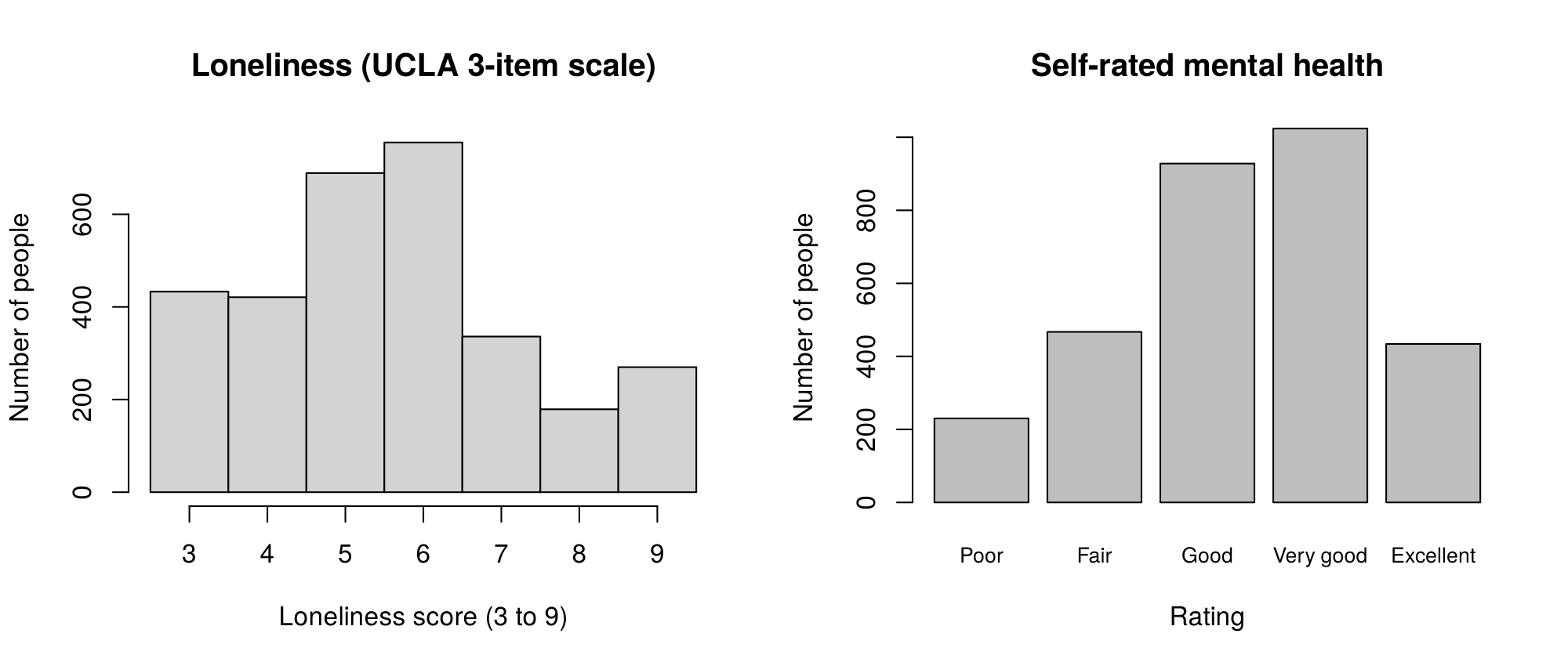
A histogram is the first look at a numeric variable, and a bar chart the first look at a categorical one. Figure 6.7 shows the histogram of the loneliness score and the bar chart of self-rated mental health, both drawn in Activity 6.2 with the functions described in 5.1.
Reading the histogram starts with its bins. The argument breaks = seq(2.5, 9.5, by = 1) sets the edges of the bins at 2.5, 3.5, 4.5 and so on, so each bar holds exactly one whole score. Without it, R chooses its own bins, which can merge two scores into one bar or leave empty gaps, and the picture of a variable with only seven values can change a good deal. The counts behind the bars, which table(brief$loneliness) prints in Activity 6.2, show that the histogram rises from 433 people at the lowest score of 3 to a peak of 755 at a score of 6, and then falls to 179 at a score of 8. The bar at 9, with 270 people, is taller than the bar at 8. A rise at the top of a scale is called a ceiling pile-up. By this we mean that a group of people chose the most extreme answer to all three items, and because the scale cannot record anything lonelier, everyone at or beyond that level receives the same score of 9. Some of these people may be far lonelier than others, but the scale cannot tell them apart, so differences among the loneliest respondents are hidden. The mean (5.57) is a little above the median (5), which reflects the longer upper tail. This happens because the mean uses the size of every value, so the higher scores in the upper tail, including the pile-up at 9, pull it upward, whereas the median depends only on the score of the person in the middle.
The bar chart is read in the order of its categories. The bars follow the order set by factor(), from Poor to Excellent, and the counts that table(brief$mental_health) prints in Activity 6.2 give their heights. Very good is the most common rating (1,024 people), followed by Good (928), and far fewer people rated their mental health as poor (230) or fair (467). If the levels had not been set, R would have placed the categories in alphabetical order (Excellent, Fair, Good, Poor, Very good), which hides the shape of an ordinal scale.
The questions behind these two readings apply to any plot of one variable, and they are worth keeping as a checklist.
A checklist for one-variable plots
For each variable, the analyst asks whether the distribution is symmetric or skewed, whether it has one peak or more, whether values pile up at the lowest or highest possible value (a floor or a ceiling), whether answers heap on round numbers, whether any value lies outside the possible range, and how many values are missing. Each answer is recorded in the analysis notes, because each one can change a later decision about summaries, recoding or models.
Two items on the checklist, values outside the possible range and answers that pile up on particular values, are the ones a numeric summary most often hides, as the next variable shows.
4.2.2 A Problem That Cleaning Left Behind: Top-Coding and Heaping
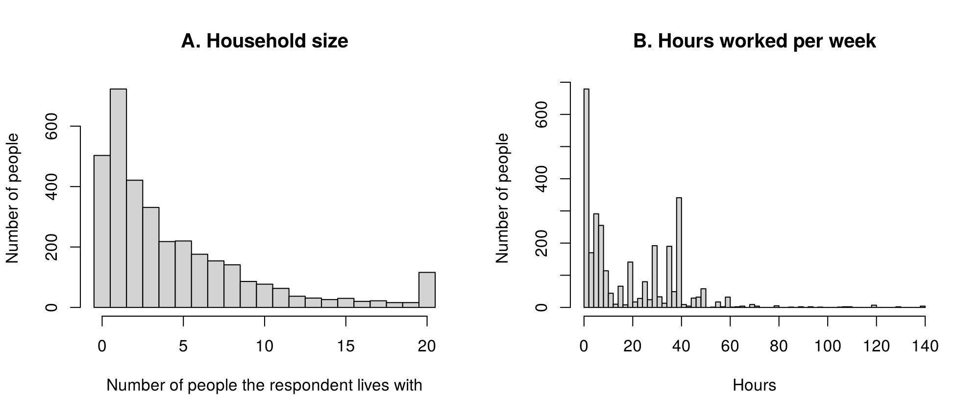
The household size variable, GEO_housing_household_size, records the number of people each respondent lives with, not counting the respondent, so 0 means living alone (503 people). The course's cleaning walkthrough used it to build a living-alone indicator, and the numeric summary that Activity 6.2 prints for it looks unremarkable: a median of 3, a mean of 4.46 and a maximum of 20. The histogram tells a different story. Panel A of Figure 6.8 shows that histogram, and panel B shows a second variable from the 2021 wave, the hours worked per week.
In panel A, the bars fall smoothly from one other person toward larger households, and then a bar of 116 people appears at exactly 20, the largest value in the data. The real distribution of household sizes does not rise again at its maximum, so the spike signals that something about the value 20 differs from the other values. Tracing the variable back to the survey explains it. Household size is the sum of eight questions that ask how many partners, children, grandchildren, parents, in-laws, siblings, roommates and other people the respondent lives with, and totals above 20 were recorded as 20. For 105 of the 116 people at 20, the eight answers added up to more than 20, and one total reached 180. Some of these answers are implausible, such as five grandchildren, five in-laws and seven siblings in one household, and they may reflect careless or mistaken responses. The summary statistics did not reveal this problem, and the histogram made it obvious. Recording every value above a limit as the limit itself is called top-coding, and its sign on a histogram is a bar at the largest value that is taller than the bars just below it, so the top value means "this much or more".
The analyst's response has three steps. The first is to check the codebook and the source questions, which is how the meaning of 20 was established. The second is to decide how the variable will be used. Used as a count, the value 20 cannot be trusted and can be set to missing with a bracket recode (Activity 6.2, question 1). Used as a grouped variable, such as living alone versus living with others, or 0, 1, 2 to 4 and 5 or more, the problem is absorbed by the top category and matters much less. The third step is to report the decision in the methods section, with the number of people affected, and, where the decision could change a result, to repeat the analysis both ways as a sensitivity analysis.
Panel B shows two further problems that the same plot can reveal. Answers to the question on hours worked per week heap on round numbers: 340 of the 2,978 people who answered reported exactly 40 hours, compared with one person at 39 and one at 41, and smaller peaks appear at 20, 30 and 35. Heaping of this kind, also called digit preference, usually reflects two habits. Many people do not know their exact hours and round them to a convenient number, and many people have a standard working week of 35 or 40 hours and report that figure even when their actual hours vary from week to week. Because of this, a reported value of 40 stands for a range of real values rather than exactly 40 hours. The consequence is that small differences in reported hours carry little information: a difference of one or two hours between two people, or between two groups, may reflect nothing more than how each person chose to round. The long right tail reaches 140 hours, and 13 people reported more than 112 hours a week, which would mean working more than 16 hours a day, every day. These values are implausible and would be checked and, in most analyses, set to missing.
4.2.3 Missing-Value Codes and Narrow Bins
A third problem can look similar on a histogram but has a different cause. Many survey files store a non-answer as a number that cannot be a real value, such as 99 for household size or 999 for hours worked, and a histogram shows such a missing-value code as a separate bar far from the rest. The numeric summary often gives a clue first. One clue is a maximum that is impossible, such as 999 hours in a week. Another is a mean that lies above the third quartile. In most variables the mean sits somewhere in the middle half of the data, between the first and third quartiles. When a few people carry a huge code such as 999, those values pull the mean far upward, because the mean adds up the size of every value. The median and the quartiles, by contrast, depend only on the order of the values, so a handful of extreme values at the top barely moves them. A mean that has risen above the third quartile is therefore a sign that a few very large values are present. The codebook confirms what the code means, and the code is then set to missing before any analysis.
Heaping and codes can be seen only when the bins are narrow enough. A bin two hours wide puts 39, 40 and 41 hours into one bar, so a pile-up at 40 disappears, and a few extreme values stretch the axis so that the bars for most people look tiny. Narrower bins, such as one bar per whole score or per hour, show both problems. In base R the bins are set with breaks, and in ggplot2 with binwidth.
Top-coding, heaping and missing-value codes each call for a different response, and treating one as another is a common error, so the rule below is worth committing to memory.
Three problems, three responses
A missing-value code is recoded to missing. A top-coded value is real but inexact, so it is kept and treated as "this much or more" (for example by using the variable in groups with a top group), and labels and the report say so. Heaping cannot be corrected, so small differences are interpreted with caution or the variable is grouped. In every case, the methods section reports the problem, the decision and the number of people affected.
Household size and working hours show that a histogram can reveal problems that summary statistics hide. The same reading of centre, spread and unusual values carries over to a numeric variable compared across groups, where the display is a set of boxplots.
4.3 Reading Boxplots Across Groups
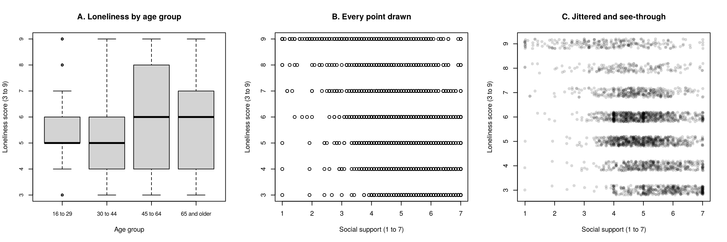
A plot of two variables shows how the variables go together. Figure 6.9 shows the boxplots of loneliness by age group (panel A) and two scatterplots of loneliness against social support (panels B and C), all drawn in Activity 6.2. Panel A is read here; panels B and C show a problem of drawing rather than of data, and they are read in 5.2.
A boxplot summarizes a numeric variable with five numbers. The thick line is the median. The box runs from the lower to the upper quartile, so it holds the middle half of the people, and its length is the interquartile range (IQR). The whiskers extend to the most extreme values that lie within 1.5 times the IQR of the box. By this we mean that R marks off a distance of one and a half box lengths beyond each end of the box, and each whisker stretches to the last actual value inside that distance. Any value beyond the whiskers is drawn as a separate point. This rule is a convention, introduced by Tukey, for flagging values that sit unusually far from the middle half of the data; it does not decide whether a value is an error. Table 6.4 gives the numbers behind panel A.
Table 6.4. The numbers behind the boxplots in panel A of Figure 6.9: the number of people, the whiskers, the quartiles and the median in each age group.
| Age group | People | Lower whisker | Lower quartile | Median | Upper quartile | Upper whisker |
|---|---|---|---|---|---|---|
| 16 to 29 | 1,079 | 4 | 5 | 5 | 6 | 7 |
| 30 to 44 | 1,060 | 3 | 4 | 5 | 6 | 9 |
| 45 to 64 | 578 | 3 | 4 | 6 | 8 | 9 |
| 65 and older | 366 | 3 | 4 | 6 | 7 | 9 |
The two older groups have a median of 6 and the two younger groups a median of 5, and the box for people aged 45 to 64 is the widest, so loneliness varies most in that group. The box for people aged 16 to 29 is narrow, because most of them scored 5 or 6. Its whiskers therefore stop at 4 and 7, and the scores 3, 8 and 9 in this group are drawn as separate points (212 people in all). These points are flagged by the 1.5 × IQR rule, and they are ordinary answers on the scale. The reason is that the rule measures distance in units of box length. Because the box for this group is very short, one and a half box lengths is also a short distance, so the whiskers stop close to the box and perfectly possible scores of 3, 8 and 9 fall beyond them. With a variable that takes only a few whole values, the points beyond the whiskers say more about the narrowness of the box than about unusual people.
The same reading applies to any boxplot. To compare groups, read the medians (the centre), the heights of the boxes and the lengths of the whiskers (the spread), and then the shape. A distribution that is skewed to the right (a long upper tail) shows a long upper whisker and a short lower one, a median near the bottom of the box, separate points above the box only, and, when the mean is marked, a mean above the median. Counts such as the number of doctor visits or days without a meal are usually right-skewed, because they cannot fall below zero but can be large, and in a skewed distribution many people are drawn beyond the upper whisker. Deciding what to do with those people is where analyses most often go wrong.
Points beyond the whiskers are flagged, not wrong
These points are flagged by the 1.5 × IQR rule, not shown to be wrong. In a skewed distribution they are often ordinary, possible values, and they may be the people who most need describing. The analyst checks any that are impossible (check, decide and report, as for the household-size spike), keeps the rest, and chooses a summary or a model that allows for a long tail, rather than deleting people to make the plot look tidier.
Exploration often points to the model as well. A count outcome that piles up at zero, has a long right tail and spreads more in groups with higher medians calls for a count model rather than linear regression. Comparing the variance of a count with its mean gives a first look at overdispersion, which means that the counts vary more than a Poisson model allows. A Poisson model assumes that the variance of a count equals its mean. So when the variance is several times the mean, the counts are much more spread out than that model expects, and a negative binomial model, which allows the variance to be larger than the mean, may be needed. This first look ignores the predictors, however. Some of the extra variation may be explained once the predictors are in the model, so the comparison is only a warning sign, and the formal checks are made on the fitted model. A predictor whose groups have clearly different medians is a candidate for the model.
Every plot read so far, from the histogram of loneliness to these boxplots, was drawn with a single line of base R code, and the next subsection turns from reading the plots to drawing them.
5.1 Drawing the Standard Plots in Base R
Base R draws a quick diagnostic plot with one line of code and needs no extra packages, which makes it the analyst's quick diagnostic tool: its plots are drawn, read and set aside, and only the useful ones are later rebuilt as polished figures with ggplot2 (Section 3). Every plotting function accepts the same labelling arguments: main for the title, xlab and ylab for the axis labels. Every plot in the briefing should carry these labels from the start, because a plot without labels is easily misread, even by the person who drew it.
Four of the functions are familiar from Lesson 2. The recall below lists them with the briefing variables to which this section applies them, and its retrieval question asks why one of them needs a helper function.
Recall: Lesson 2, Section 3 (Activity 2.3: describe the course data and check the scales)
Activity 2.3 in Lesson 2, Section 3 drew four standard plots with base R: hist(x) for a histogram of one numeric variable, barplot(table(x)) for a bar chart of one categorical variable, boxplot(y ~ group, data = ...) for boxplots of a numeric variable across groups, and plot(x, y) for a scatterplot of two numeric variables. This section applies the same four functions to the briefing file: the loneliness score, self-rated mental health, loneliness by age group, and loneliness against social support.
Retrieval question. Why is barplot() given table(x) and not the raw variable?
barplot() draws one bar for each number it is given, so it needs counts. table(x) counts the people in each category, and barplot() then draws one bar per count.Reading the code of these functions follows the same logic as reading the plots. In hist(brief$loneliness, breaks = seq(2.5, 9.5, by = 1)), the variable goes along the horizontal axis and breaks fixes one bar per score (4.2.1). In barplot(table(brief$mental_health)), the bars follow the order of the factor levels. In boxplot(loneliness ~ age_group, data = brief), the variable before the tilde runs up the vertical axis and there is one box for each group named after it. In plot(brief$support, brief$loneliness), the first variable goes along the horizontal axis and the second up the vertical axis, with one point per person.
One function is new in this lesson. The function pairs() draws a scatterplot matrix, a small scatterplot for every pair of the chosen variables, with the variable names on the diagonal. Each panel is a quick look at one pair, and the panel above the diagonal shows the same pair as the panel below it with the axes swapped. With 3,083 people and scores that take few values, the panels are crowded, so the matrix is best used to spot strong patterns or unexpected shapes, after which a single scatterplot or a correlation heatmap (Section 4) gives a clearer view. Figure 6.10 shows the scatterplot matrix that Activity 6.2 draws for loneliness, support, depression and age.
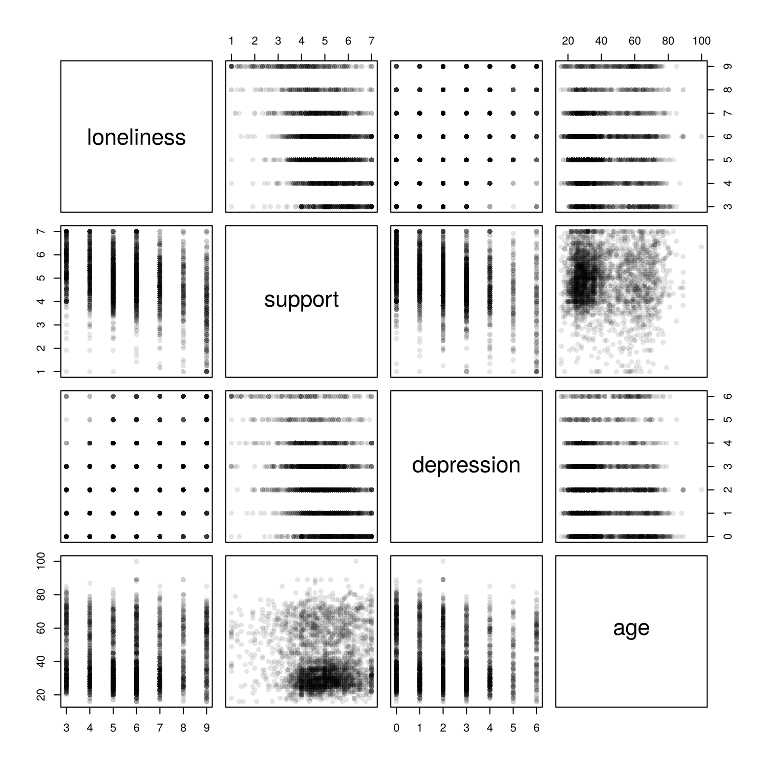
pairs() for four briefing variables (n = 3,083). Each off-diagonal panel is a scatterplot of the two variables named in its row and column.The panels of Figure 6.10 that involve loneliness or depression look like grids of dots, because both scores take only a few whole values. The same problem affects the single scatterplot in panel B of Figure 6.9, and the next subsection explains how to fix it.
5.2 Jitter and Transparency for Overplotted Points
Panel B of Figure 6.9 draws one solid point for each of the 3,083 people. Because the loneliness score takes only seven values, the points fall on seven horizontal lines and cover one another, a problem called overplotting, and the plot cannot show where most people are. Panel C applies two remedies. The function jitter() adds a small random amount to each value so that points sharing a value spread out a little, and col = rgb(0, 0, 0, 0.15) draws each point in black at 15% opacity, so that areas where many points overlap look darker. The function set.seed() fixes the random numbers, so the jittered plot is the same each time the code runs. Jitter changes only the picture. By this we mean that the random shift is applied to where each point is drawn, not to the values stored in the data, so any mean, correlation or model calculated afterwards uses the original scores. The shift is also kept small, less than half the gap between neighbouring scores, so each point stays closer to its true value than to any other value and the plot can still be read correctly. Panel C shows that most people have support scores between 4 and 6 and loneliness scores of 5 or 6, and that people with more support tend to report less loneliness.
Jitter and transparency make the scatterplots readable without altering a single value. With every display now drawn and readable, the last step is to arrange the plots and keep them.
5.3 Several Plots in One Window, and Saving Plots
The setting par(mfrow = c(rows, columns)) divides the plotting window into a grid, and each new plot fills the next cell, row by row. par(mfrow = c(1, 2)) places two plots side by side, and par(mfrow = c(2, 2)), used in the Anscombe activity, places four in a square. The setting stays in force until it is changed, so the code resets it with par(mfrow = c(1, 1)) afterwards.
Plots in the RStudio Plots pane disappear when the session ends. To keep a plot, the analyst sends it to a file. The function png("name.png", width = 1600, height = 800, res = 200) opens an image file 1,600 pixels wide and 800 pixels high, at a resolution of 200 pixels per inch, which prints at 8 by 4 inches. Every plot drawn afterwards goes into the file and does not appear on screen. The function dev.off() closes the file, which saves it in the working directory. The functions pdf() and jpeg() work in the same way for other formats, and the Export button in the Plots pane saves a plot by hand. Saving with code is better practice, because the code records exactly how the figure was made and remakes it in one step if the data change.
Before you run the activity for this section, you may find it helpful to watch the code run. The card below links to a narrated R walkthrough of the base R plots in this section and the ggplot2 plots in Section 3.
Narrated R walkthrough: Data Visualization in Base R and ggplot2
The walkthrough runs the code from this section and the next one line at a time, draws each plot as the line runs, and explains every argument. It is a good place to start if the activities feel fast.
Open the walkthroughActivity 6.2 carries out every step of this section in R. It loads the survey and builds the briefing file (4.1), draws the histogram and the bar chart and finds the spike in household size (4.2), compares loneliness across age groups with boxplots (4.3), draws the scatterplots with and without jitter and the scatterplot matrix (5.1 and 5.2), and saves two plots side by side to a file (5.3). Download the code and run it along with the text version below; its preparation code is the starting point for every later activity in this lesson.
Text version of the activity: the code of the run-along script, its console output and notes on reading it.
load(url("https://raw.githubusercontent.com/jorgeandr3s/heal/main/cscs/public_data/CSCS2025_full_cleaned_deidentified_data_and_metadata.RData"))   # survey data, read from the web
data <- data[data$SURVEY_collection_year == 2021, ]   # the 2021 wave: one row per person
nrow(data) # how many people?The file adds three objects to the environment, and the one called data holds the survey responses. The square brackets keep the rows from the 2021 wave and every column. The 2021 wave holds 4,045 people.
data$loneliness <- data$LONELY_ucla_loneliness_scale_score   # 3 to 9, higher = lonelier
data$support    <- data$PSYCH_zimet_multidimensional_social_support_scale_score   # 1 to 7
data$depression <- data$WELLNESS_phq_score                   # 0 to 6
data$anxiety    <- data$WELLNESS_gad_score                   # 0 to 6
data$life_sat   <- data$WELLNESS_life_satisfaction_num       # 1 to 10
data$age        <- data$DEMO_age                             # years
data$gender <- as.character(data$DEMO_gender)
data$gender[data$gender == "Presented but no response"] <- NA
data$gender <- factor(data$gender, levels = c("Woman", "Man", "Non-binary"))
data$mental_health <- as.character(data$WELLNESS_self_rated_mental_health)
data$mental_health[data$mental_health == "Presented but no response"] <- NA
data$mental_health <- factor(data$mental_health,
  levels = c("Poor", "Fair", "Good", "Very good", "Excellent"))
data$age_group[data$age < 30] <- "16 to 29"
data$age_group[data$age >= 30 & data$age < 45] <- "30 to 44"
data$age_group[data$age >= 45 & data$age < 65] <- "45 to 64"
data$age_group[data$age >= 65] <- "65 and older"
data$age_group <- factor(data$age_group,
  levels = c("16 to 29", "30 to 44", "45 to 64", "65 and older"))
brief <- na.omit(data[, c("loneliness", "support", "depression", "anxiety",
                          "life_sat", "age", "age_group", "gender", "mental_health")])
c(kept = nrow(brief), left_out = nrow(data) - nrow(brief)) # people kept and left outEach bracket recode changes only the rows that meet the condition inside the brackets. The first age-group line, for example, writes "16 to 29" into age_group for every person whose age is below 30, and factor() with levels fixes the order of the categories. na.omit() then keeps the people with no missing value on the nine briefing variables, and the last line prints how many were kept (3,083) and how many of the 4,045 respondents were left out (962), which the briefing should report.
summary(brief$loneliness)                  # a numeric summary first
table(brief$loneliness)                    # the counts the bars will show
hist(brief$loneliness, breaks = seq(2.5, 9.5, by = 1),   # one bar for each score
     main = "Loneliness (UCLA 3-item scale)",
     xlab = "Loneliness score (3 to 9)", ylab = "Number of people")
table(brief$mental_health)                 # the counts the bars will show
barplot(table(brief$mental_health), main = "Self-rated mental health",
        xlab = "Rating", ylab = "Number of people")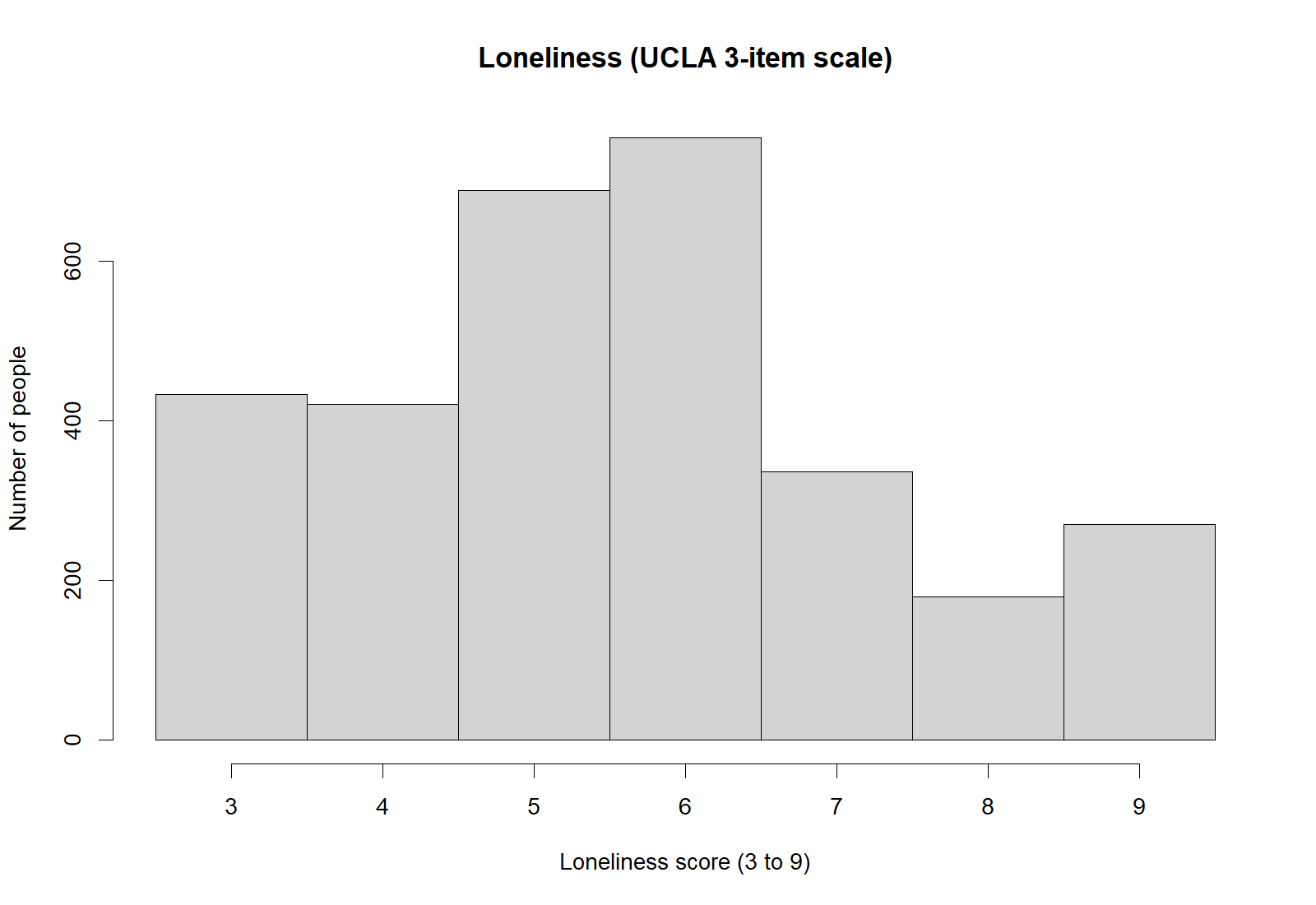
The scores run from 3 to 9, the median is 5 and the mean is 5.57. The most common scores are 6 (755 people) and 5 (689). The bar at 9, the highest possible score (270 people), is taller than the bar at 8 (179): a ceiling pile-up. The bar chart follows the order set by factor(), from Poor to Excellent: Very good is the most common rating (1,024 people), and far fewer people rated their mental health as poor (230) or fair (467).
summary(data$GEO_housing_household_size)   # people each respondent lives with
hist(data$GEO_housing_household_size, breaks = seq(-0.5, 20.5, by = 1),
     main = "Household size",
     xlab = "Number of people the respondent lives with", ylab = "Number of people")
sum(data$GEO_housing_household_size == 20, na.rm = TRUE)   # how many at the top value?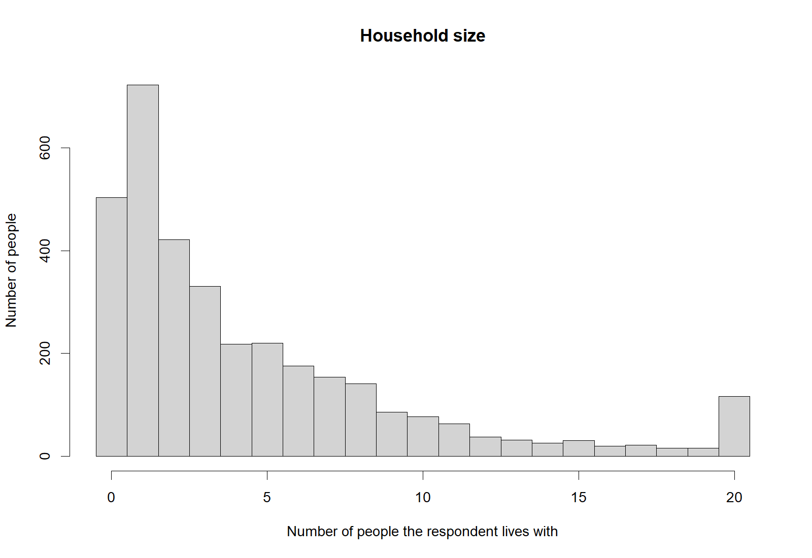
The summary uses the full 2021 wave, in which 618 people did not answer the household questions, and nothing in it looks unusual. The histogram (above) rises again at 20, the largest value, and sum(... == 20, na.rm = TRUE) counts the 116 people there. The argument na.rm = TRUE tells sum() to skip missing values, which would otherwise make the result NA.
boxplot(loneliness ~ age_group, data = brief, main = "Loneliness by age group",
        xlab = "Age group", ylab = "Loneliness score (3 to 9)")
tapply(brief$loneliness, brief$age_group, median)   # the thick line in each box
tapply(brief$loneliness, brief$age_group, IQR)      # the length of each box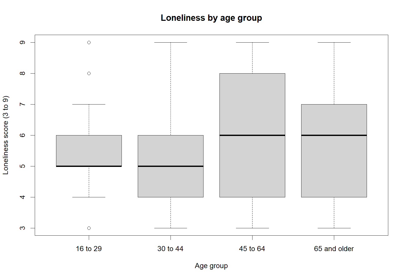
The formula loneliness ~ age_group draws one box for each age group. tapply() applies median() and IQR() to the loneliness scores within each group: the medians (the thick lines) are 5, 5, 6 and 6, and the boxes are 1, 2, 4 and 3 points long.
plot(brief$support, brief$loneliness,                  # every person as one point
     xlab = "Social support (1 to 7)", ylab = "Loneliness score (3 to 9)")
set.seed(2021)                                         # the same jitter every time
plot(jitter(brief$support), jitter(brief$loneliness),  # nudge each point a little
     pch = 16, col = rgb(0, 0, 0, 0.15),               # small grey see-through dots
     xlab = "Social support (1 to 7)", ylab = "Loneliness score (3 to 9)")
pairs(brief[, c("loneliness", "support", "depression", "age")],
      pch = 16, col = rgb(0, 0, 0, 0.1))               # every pair in one grid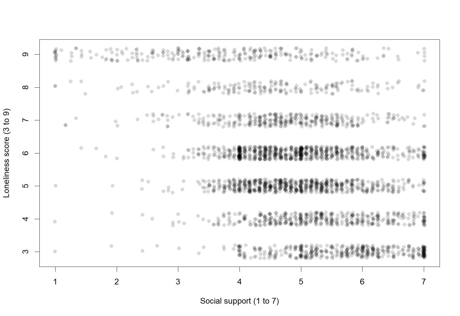
These lines draw three plots and print nothing. The first shows seven solid stripes. The second (above) uses jitter(), small filled dots (pch = 16) and a see-through grey (rgb(0, 0, 0, 0.15), where the last number is the opacity), so the dense areas look darker; set.seed(2021) makes the random jitter the same each time. pairs() draws one panel for every pair of the four variables, with the variable names on the diagonal.
png("briefing_base_r.png", width = 1600, height = 800, res = 200)   # open a file
par(mfrow = c(1, 2))                       # one row, two plots
hist(brief$loneliness, breaks = seq(2.5, 9.5, by = 1),
     main = "A. Loneliness", xlab = "Loneliness score", ylab = "Number of people")
boxplot(loneliness ~ age_group, data = brief,
        main = "B. Loneliness by age group", xlab = "Age group", ylab = "Loneliness score")
par(mfrow = c(1, 1))                       # back to one plot per window
dev.off()                                  # close the file, which saves it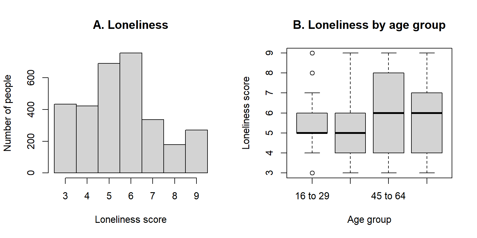
Nothing appears in the Plots pane, because png() sent both plots to the file briefing_base_r.png in R's working directory (the image above). The message after dev.off() names the graphics device R returned to: this recording printed png 2, and in RStudio it reads RStudioGD 2 or null device 1, depending on whether other plots are open. It can be ignored.
R Reflect on what you just ran
Answer each question from your own output, as on the final exam: read the plot, name the problem, and say what the analyst should do.
1. For each of your two histograms (loneliness and household size), name the problem it reveals that its summary did not make obvious. What should the analyst do about the 116 people at 20 before any analysis, and what should be reported?
sum() gives the number of people affected (116). Decide: used as a count, 20 cannot be trusted and is set to missing with a bracket recode (data$household <- data$GEO_housing_household_size, then data$household[data$household == 20] <- NA); used in groups with a top group (for example 0, 1, 2 to 4, and 5 or more), it is kept as "5 or more" and the problem matters much less. Report: the methods section states the problem, the decision and the number of people affected (116), and the analysis is repeated both ways as a sensitivity analysis if the decision could change a result.2. Describe what the boxplots and the output of lines 55 and 56 show about the centre and the spread of loneliness across the four age groups. Several scores in the youngest group are drawn as points beyond the whiskers. Should these people be removed from the analysis? Explain.
3. Run your own code: at the end of the script, type plot(jitter(brief$depression), jitter(brief$loneliness), pch = 16, col = rgb(0, 0, 0, 0.15)) and run it. Both scores take only seven whole values. Why are the points jittered and drawn partly transparent, and what does jitter leave unchanged? What does your plot show about how loneliness is related to depression? Why is it better to save a figure with code, as lines 69 to 76 do, than to export it by hand?
rgb(0, 0, 0, 0.15) is the opacity) makes crowded areas darker, so the plot shows where most people are. Jitter changes only the picture: the values in brief, and any correlation or model computed from them, stay the same. The plot shows that loneliness tends to be higher among people with more depressive symptoms: people with no symptoms cluster at the lowest loneliness score (3), the darkest areas at depression scores of 2 and 3 are at loneliness scores of 5 and 6, and at the top of the depression scale (6) loneliness piles up at 9, although people vary widely at every level. Saving a figure with code, as lines 69 to 76 do, is better than exporting it by hand, because the code records exactly how the figure was made and remakes it in one step if the data change.Your output reproduces the numbers read in this section, from the 962 people left out of the briefing file to the 116 households recorded at 20, and the questions ask you to apply check, decide and report to them and to explain what jitter changes and what it leaves alone.
This section has prepared the briefing file, read histograms and boxplots for data problems and group differences, and drawn, arranged and saved the base R plots behind those readings. The key takeaways below summarize these steps, the knowledge check reviews them, and Section 3 rebuilds the most useful plots as polished figures with ggplot2.
Key Takeaways
- 4.1 Every plot in the briefing comes from one analysis file,
brief, prepared in base R. Bracket recoding changes only the rows that meet the condition inside the square brackets (for example, setting the answer "Presented but no response" toNA),factor()withlevelsfixes the order of the categories, andna.omit()keeps only the people with no missing value on the chosen variables, the complete cases. A single complete-case file means that every panel describes the same people, which makes the panels comparable. The cost is that the figures describe only people who answered every question, and those people may differ from the ones who skipped some. So whenever you seena.omit(), read from the row counts that R prints before and after the step (for example withnrow()) how many people were kept and how many were dropped, and say so in the report: here 3,083 of 4,045 respondents were kept and 962 (24%) were left out for missing data. - 4.2 A histogram is your first look at one variable, and with bins narrow enough (one bar per whole score, set with
breaksin base R orbinwidthin ggplot2) it shows problems that a numeric summary hides. Look for skew; a pile-up at the top or bottom of a scale (a ceiling or floor, such as the 270 people at the loneliness maximum of 9); heaping on round numbers (340 people reporting exactly 40 hours of work); top-coding, where a bar at the largest value is taller than the bars just below it because every larger value was recorded as that value (the 116 households at 20, meaning "20 or more"); values outside the possible range; and a separate bar far from the rest, which may be a missing-value code such as 99 or 999. The numeric summary often gives the first clue, with an impossible maximum or a mean that sits above the third quartile. Respond to each problem in three steps: check the codebook and the source questions, decide how to handle it, and report the decision and the number of people affected in the methods. As 4.2.3 sets out, a missing-value code is recoded toNA, a top-coded value is real but inexact and is usually kept as "this much or more" (for example by grouping the variable), and heaping cannot be corrected, so small differences are interpreted with caution. - 4.3 A boxplot summarizes a numeric variable in a few numbers: the thick line is the median, the box runs from the lower to the upper quartile and so holds the middle half of the people (its length is the interquartile range, or IQR), the whiskers reach the most extreme values within 1.5 times the IQR of the box, and anything beyond them is drawn as a separate point. To compare groups, read the medians for the centre, the box heights and whisker lengths for the spread, and then the shape; in Figure 6.9, for example, the two older age groups have a median of 6 and the two younger groups a median of 5. Right skew shows as a long upper whisker and a short lower one, a median near the bottom of the box, separate points above the box only, and a mean above the median when the mean is marked. Points beyond the whiskers are flagged by the 1.5 × IQR rule, not shown to be wrong (in the narrow box for people aged 16 to 29, ordinary scores of 3, 8 and 9 are drawn as points), so check any that are impossible and keep the rest rather than deleting people to tidy the plot. If the outcome is a right-skewed count whose variance is several times its mean, say that this first look points to a count model, possibly a negative binomial model, rather than linear regression.
- 5.1 Base R is the analyst's quick diagnostic tool: each standard plot takes one line of code, and you draw it, read it and move on.
hist(x)draws a histogram of one numeric variable;barplot(table(x))draws a bar chart, and thetable()step is needed becausebarplot()draws one bar for each number it is given, so it needs counts;boxplot(y ~ group, data = ...)draws one box per group;plot(x, y)draws a scatterplot; andpairs()draws a scatterplot matrix, with one small scatterplot for every pair of the chosen variables. Give every plot a title and axis labels from the start withmain,xlabandylab, because an unlabelled plot is easily misread, even by the person who drew it. When a question shows a line of base R code, say which plot it draws and which variable goes where; inboxplot(loneliness ~ age_group, data = brief), for example, loneliness runs up the vertical axis and there is one box for each age group. - 5.2 When many people share a small number of values, such as a loneliness score with only seven possible values, their points are drawn on top of one another (overplotting), and a row of five people looks the same as a row of five hundred. Jitter adds a small random shift to each point so that points sharing a value spread out a little, and transparency (
col = rgb(0, 0, 0, 0.15)in base R, oralphain ggplot2) makes crowded areas look darker, so together they show where most people are. They change only the picture: the data, and anything calculated from them, stay exactly the same, andset.seed()makes the random jitter the same each time the code runs. When asked why a figure uses jitter and transparency, name the shared values that cause the overlap, and say that the fix changes where the points are drawn, not the data or any fitted line. - 5.3
par(mfrow = c(rows, columns))divides the plotting window into a grid that fills row by row, soc(1, 2)puts two plots side by side andc(2, 2)puts four in a square; the setting stays in force until you reset it withpar(mfrow = c(1, 1)). To keep a plot, send it to a file:png("name.png", width = 1600, height = 800, res = 200)opens the file, every plot drawn next goes into it rather than onto the screen, anddev.off()closes the file and saves it in the working directory. A common surprise is that nothing appears in the Plots pane afterpng(); that is expected, andgetwd()tells you where the file went. Saving with code is better than clicking Export, because the code records exactly how the figure was made and remakes it in one step if the data change. The printed size follows from the pixels and the resolution, so a file of 1,600 by 800 pixels at 200 pixels per inch prints at 8 by 4 inches.
1. A community health survey has 2,500 respondents. The analyst builds the analysis file with dat <- na.omit(survey[, vars]), where vars names the eight variables used in the figures, and prints the output below. Which sentence should the report include?
> nrow(survey)
[1] 2500
> nrow(dat)
[1] 1900
> nrow(survey) - nrow(dat)
[1] 600
> round(100 * nrow(dat) / nrow(survey))                    # percentage kept
[1] 76
> round(100 * (nrow(survey) - nrow(dat)) / nrow(survey))   # percentage dropped
[1] 24
na.omit() does and the counts that R prints. It keeps only the rows with no missing value on the chosen variables, so the output shows that 1,900 respondents were kept and 600 were dropped, and its last two lines give these as 76% and 24% of the 2,500. Every panel then describes the same 1,900 people, and the report gives both numbers because people who skip questions can differ from those who answer them all. The option claiming the figures are free of bias is tempting, but keeping only complete cases can introduce bias rather than remove it, which is exactly why the number excluded is reported. (Section 2, 4.1 Preparing the Briefing File, Who is left out?; Objective 4.1)2. In a survey of 800 students, the question on days of school missed in the past 30 days gives the output below. The codebook has not yet been checked. What do these clues suggest, and what should the analyst do?
> summary(dat$days_missed)
   Min. 1st Qu.  Median    Mean 3rd Qu.    Max.
  0.000   0.000   1.000   3.744   3.000  99.000
> sum(dat$days_missed == 99)
[1] 12
3. Boxplots compare waiting times at three walk-in clinics, and the table gives the numbers behind each box (in minutes). A manager proposes deleting the patients drawn beyond the whiskers before the clinics are compared. Which reading of the boxplots, and which reply to the manager, is correct?
| Clinic | Patients | Lower whisker | Lower quartile | Median | Upper quartile | Upper whisker | Points beyond the whiskers |
|---|---|---|---|---|---|---|---|
| North | 210 | 5 | 15 | 20 | 30 | 52 | 6 points, 55 to 95 |
| South | 180 | 10 | 25 | 35 | 50 | 85 | 3 points, 90 to 120 |
| East | 95 | 5 | 10 | 15 | 20 | 35 | 4 points, 40 to 70 |
4. In a survey of 2,400 adults, the number of close friends (whole numbers from 0 to 10) is plotted against a wellbeing score (whole numbers from 1 to 7). With solid points the plot is a regular grid of dots, and a combination held by hundreds of people looks the same as one held by a single person. The analyst redraws it with the code below. Which statement about the new plot is correct?
plot(jitter(dat$friends), jitter(dat$wellbeing), pch = 16, col = rgb(0, 0, 0, 0.15),
     xlab = "Number of close friends (0 to 10)", ylab = "Wellbeing score (1 to 7)")
jitter() adds a small random amount to where each point is drawn, pch = 16 draws small filled dots, and the last number in rgb(0, 0, 0, 0.15) is the opacity (15%), so areas where many points overlap build up into darker patches that show where most people are. The first option is tempting, but jitter() is applied inside plot() to the positions drawn; the columns in dat, and any correlation or model computed from them, do not change. (Section 2, 5.2 Jitter and Transparency for Overplotted Points; Objective 5.2)5. An analyst runs the code below. Afterwards, the RStudio Plots pane is empty. Which statement is correct?
png("clinic_waits.png", width = 1600, height = 800, res = 200)
par(mfrow = c(1, 2))
hist(dat$wait, main = "A. Waiting time", xlab = "Minutes", ylab = "Number of patients")
boxplot(wait ~ clinic, data = dat, main = "B. Waiting time by clinic",
        xlab = "Clinic", ylab = "Minutes")
par(mfrow = c(1, 1))
dev.off()
png() opens an image file 1,600 by 800 pixels at 200 pixels per inch (1,600 / 200 = 8 and 800 / 200 = 4 inches), so everything drawn next goes to the file and not to the screen; par(mfrow = c(1, 2)) divides the page into one row and two columns; hist() draws a histogram of one numeric variable and boxplot(wait ~ clinic, ...) draws one box per clinic; and dev.off() closes the file, which saves it in the working directory. The stacked option reverses the order: the first number in mfrow is the number of rows. Saving with code is better than exporting by hand because the script records exactly how the figure was made and remakes it in one step if the data change. (Section 2, 5.1 Drawing the Standard Plots in Base R and 5.3 Several Plots in One Window, and Saving Plots; Objectives 5.1 and 5.3)6. A provincial survey asked 2,400 students how many sugary drinks they had in the past week. The codebook says that answers above 21 were recorded as 21 and that 99 means "don't know". The analyst prints the output below. How should the two values be handled?
> sum(dat$drinks == 99)
[1] 96
> sum(dat$drinks == 19)
[1] 2
> sum(dat$drinks == 20)
[1] 4
> sum(dat$drinks == 21)
[1] 41
dat$drinks[dat$drinks == 99] <- NA. The 41 students at 21, far more than the 2 at 19 and the 4 at 20, are the sign of top-coding: these students did answer, and 21 means "21 or more", so they are kept, the top value is labelled that way or the variable is used in groups with a top group, and the methods state the number affected. The first option is tempting because both values come from the codebook, but setting the top-coded students to missing would drop the heaviest drinkers, whose answers are real. (Section 2, 4.2.2 A Problem That Cleaning Left Behind: Top-Coding and Heaping, and 4.2.3 Missing-Value Codes and Narrow Bins; Objective 4.2)The Grammar of Graphics with ggplot2
Data, a mapping, a geom and labels
| Line of code | Part of the grammar |
|---|---|
ggplot(brief, aes(x = loneliness)) + | Data and the aesthetic mapping |
geom_histogram(binwidth = 1, fill = "#0B7B6B", colour = "white") + | The geom, with fixed (set) colours |
labs(title = "...", x = "...", y = "...") | Labels |
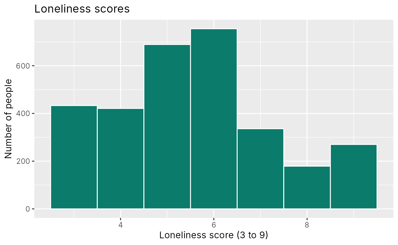
geom_bar() counts; geom_col() draws values
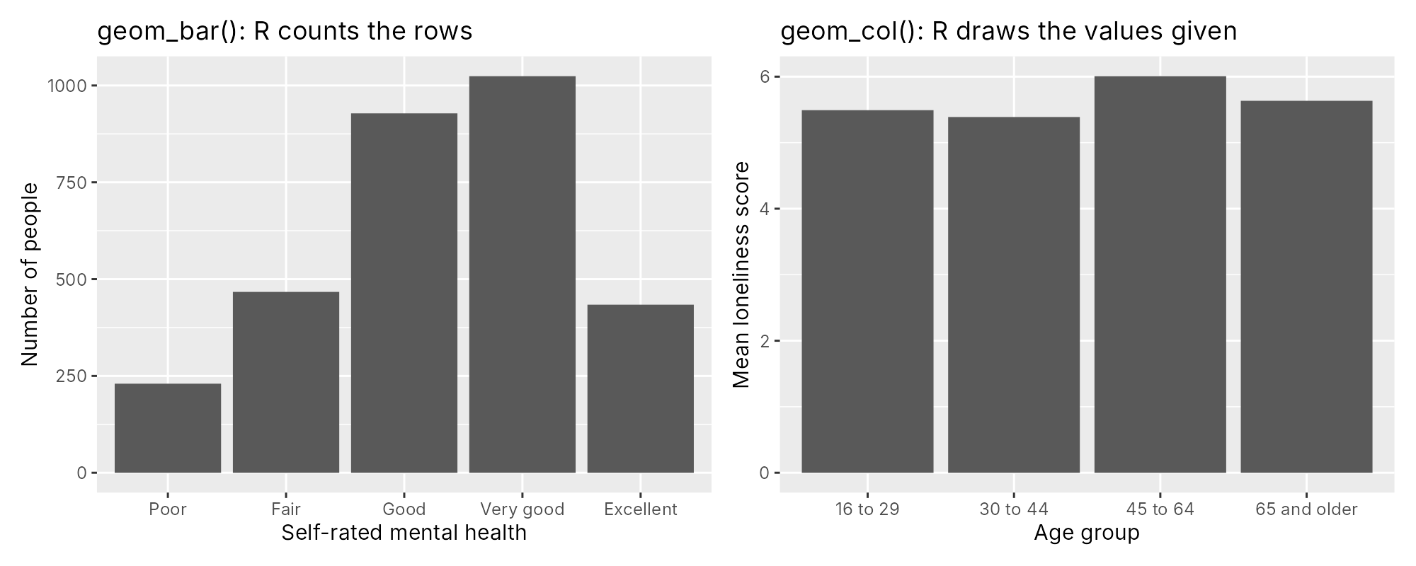
A boxplot with every person shown
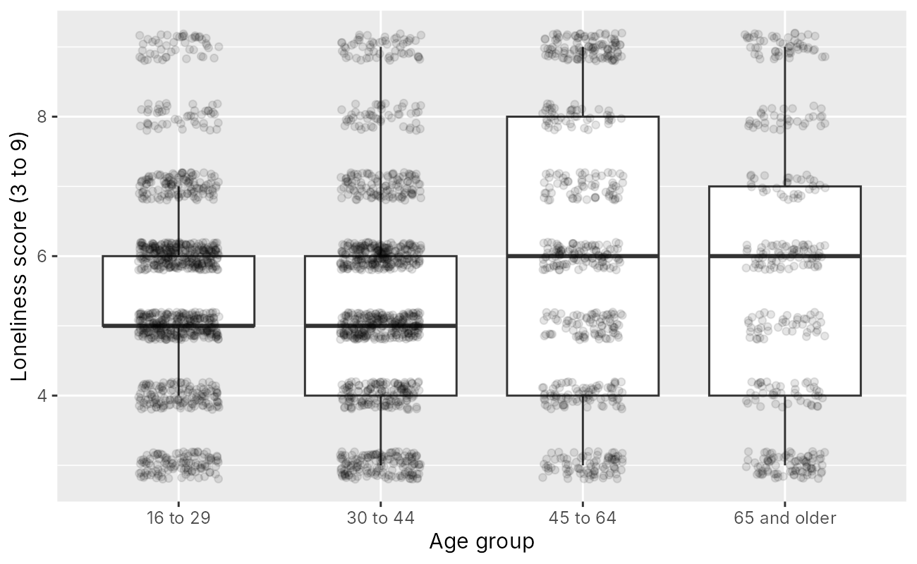
geom_boxplot() and geom_jitter() (n = 3,083).Loneliness across age, with a loess curve
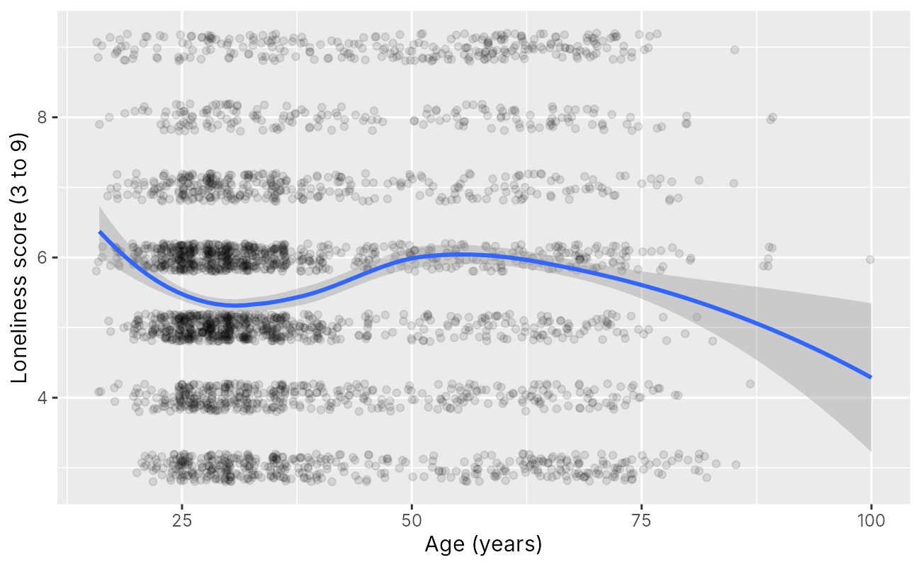
Small multiples with facet_grid()
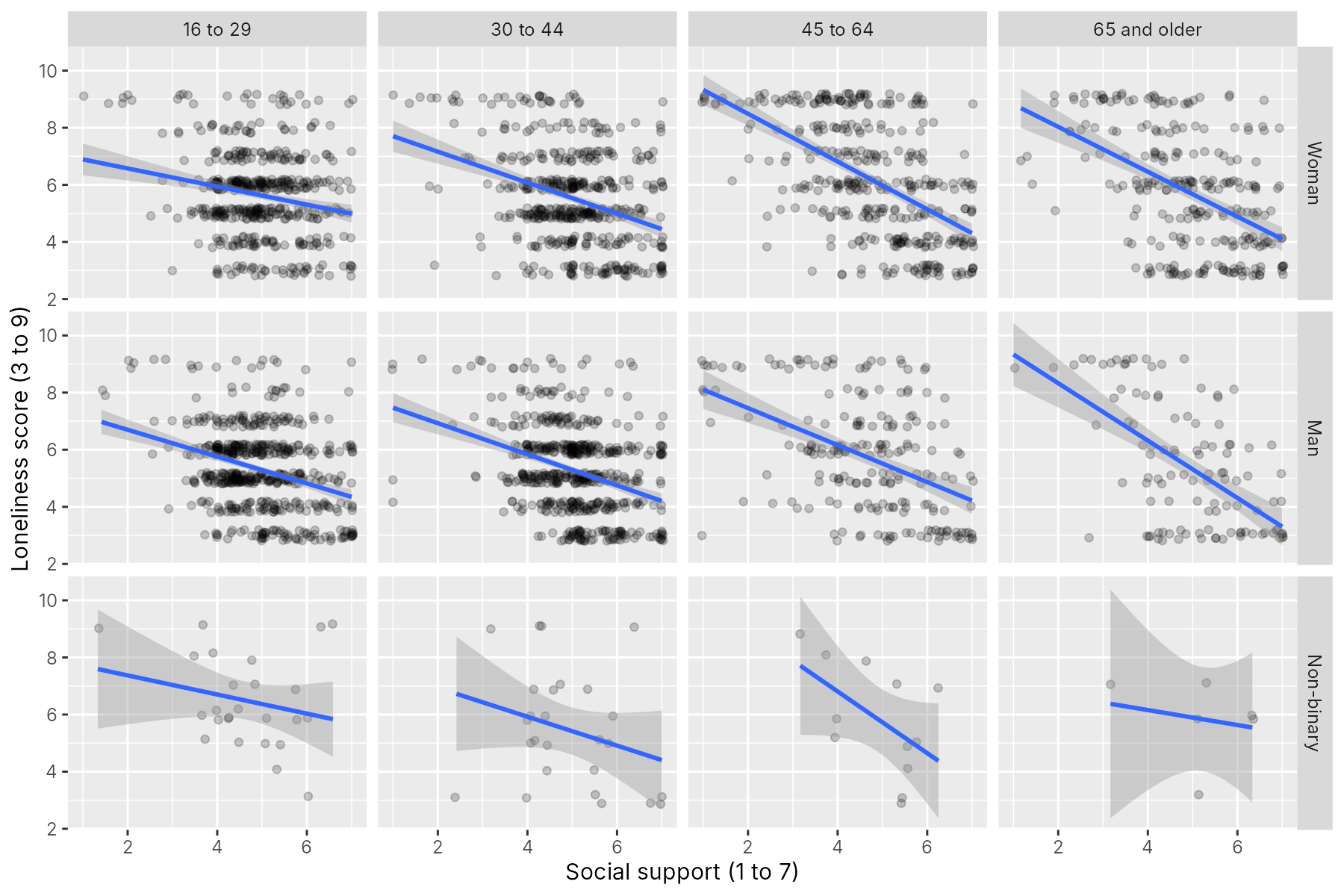
A colour-blind-safe palette
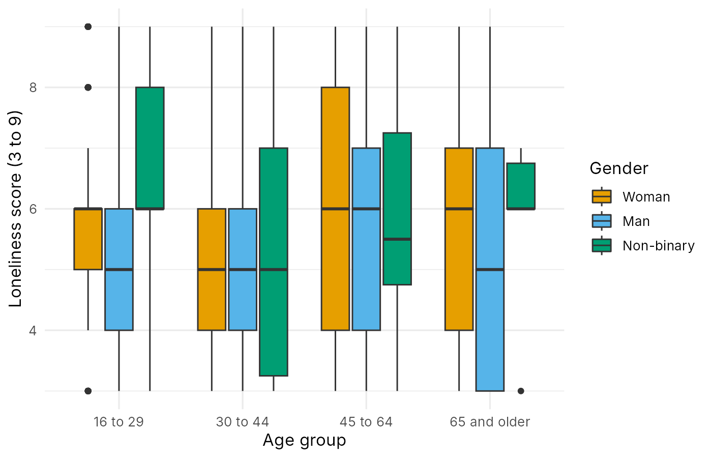
theme_minimal().Overview
Base R plots are quick to draw, and Section 2 used them to check the data. A figure for the working group's briefing, or for a manuscript, needs more care: consistent labels, readable colours, panels that share a scale, and a file of the right size and resolution. The ggplot2 package (Wickham, 2016) is the most widely used tool in R for such figures. It belongs to the tidyverse, a family of R packages for working with data. The walkthroughs and this lesson keep data preparation in base R, exactly as in Section 2, and ggplot2 is the tidyverse package that this lesson uses for figures. This section describes the grammar on which ggplot2 is built and how to read a figure's code in plain words. It then builds the core displays, separates the two geoms that draw bars, reads a scatterplot with a smoother, compares groups with facets, and makes a figure readable for every reader with a colour-blind-safe palette and a theme before saving it to a file.
Learning Objectives
- 5.4 Describe the layered grammar of graphics in terms of data, aesthetics, geoms, scales, facets and themes, and say in plain words what each line of a ggplot2 figure's code does for the figure.
- 5.5 Build a histogram, a bar chart, a boxplot with jittered points, and a scatterplot with a smoother in ggplot2.
- 5.6 Distinguish
geom_bar(), which counts rows, fromgeom_col(), which draws supplied values. - 5.7 Read a scatterplot with a loess or straight line: describe the pattern, say what the grey 95% confidence band shows, and say where the line deserves the least trust.
- 5.8 Compare a display across groups with
facet_wrap()andfacet_grid(), choose between colour and facets, and say when a panel holds too few people to interpret. - 5.9 Apply a colour-blind-safe palette and a theme, add a second cue that survives greyscale printing, and save a figure with
ggsave().
5.4 The Layered Grammar of Graphics
5.4.1 Six Parts of Every Plot
Leland Wilkinson described a grammar of graphics in which every statistical graphic is assembled from a small set of independent parts, in the way that a sentence is assembled from parts of speech (Wilkinson, 2005). By this we mean that a chart is not treated as a fixed type, such as "a bar chart" or "a scatterplot", but as a combination of separate choices: which data are used, which variables are placed on which axes or given which colours, what kind of mark is drawn, and so on. Changing one choice while keeping the others gives a different chart. For example, loneliness by age group drawn with boxes gives boxplots, and the same variables on the same axes drawn with jittered points show every person instead. Hadley Wickham adapted the idea into a layered grammar, in which a plot is built by adding layers one at a time, and implemented it as ggplot2 (Wickham, 2010). The practical benefit is that one template covers almost every display: once the parts are familiar, a histogram, a boxplot and a faceted scatterplot differ only in a line or two of code.
Figure 6.11 lists the six parts of a ggplot2 plot, each with an example taken from the briefing.
The six flip cards below expand the parts named in Figure 6.11. Click each card to read what the part does and which code controls it; the cards also serve as a reference while you run Activity 6.3.
Of the six parts, the data, the aesthetics and the geoms are needed for every plot, while scales, facets and the theme have sensible defaults and are changed only when needed. The distinction between mapping a variable inside aes() and setting a fixed value outside it, explained on the Aesthetics card, is the one that matters most when reading code.
5.4.2 The ggplot2 Template
The parts are joined into a single block of code by one template, shown as Equation 6.1. The function ggplot() receives the data and the aesthetic mappings, and each further part is added with a plus sign at the end of the line before it:
geom_...() +
labs(title = ..., x = ..., y = ...) +
theme_...()Eq 6.1
Three errors are common when the template in Equation 6.1 is first used. Expand the panel below to read each error, the message or symptom it produces, and its remedy.
The package is not loaded. The message could not find function "ggplot" means that library(ggplot2) has not been run in this session. The package is installed once with install.packages("ggplot2"), and loaded with library(ggplot2) in every new session.
The plus sign starts a line. R reads each line as a complete command when it can. If a line ends without a plus sign, R draws the plot so far and then treats the next line, starting with +, as a separate command, which gives an error. The plus sign therefore goes at the end of a line, never at the start of the next.
A fixed colour is put inside aes(). Writing aes(colour = "blue") maps the word "blue" as if it were a variable, so the points are drawn in a default colour with a legend that says "blue". A fixed colour belongs outside aes(), as in geom_point(colour = "blue").
Each of these errors comes from the structure of the template: the package must be loaded, each plus sign ends a line, and only variables go inside aes().
5.4.3 Reading a Figure's Code in Plain Words
Knowing the parts of a plot also makes it possible to read code written by someone else, which is how a figure is checked. You do not need to remember function names to read ggplot2 code: ask of each line what it adds to the picture. Table 6.5 reads one block of code in this way. The code draws loneliness against social support with a straight line for each gender, in one panel per age group, and the rest of this section builds each of its layers in turn.
Table 6.5. Reading a figure's code line by line in plain words.
| Line of code | What it does for the figure |
|---|---|
ggplot(brief, aes(x = support, y = loneliness, colour = gender)) | Uses the briefing file, puts support across the bottom and loneliness up the side, and gives each gender its own colour for points and lines, with a legend. |
geom_jitter(height = 0.2, alpha = 0.15) | Draws one point per person, nudged slightly up or down and drawn see-through, so people with the same scores do not hide one another and crowded areas look darker. |
geom_smooth(method = "lm") | Adds a straight line of average loneliness across support for each colour group, with a grey 95% confidence band around it (method = "loess" would draw a curve that can bend). |
facet_wrap(~ age_group) | Splits the figure into one panel per age group, on the same axes, so the groups can be compared side by side. |
labs(x = "Social support (1 to 7)", y = "Loneliness score (3 to 9)", colour = "Gender") | Replaces R names with plain axis titles that give the range, and titles the legend. |
theme_minimal() | Gives the figure a plain white background with light grid lines. |
Reading the finished figure then follows the same order: what the axes show, what the colours and panels separate, what the lines and bands say about the average, and how many people sit behind each panel. With the template and this way of reading code in hand, the next subsection builds the displays that Section 2 drew in base R.
5.5 Building the Core Displays in ggplot2
5.5.1 One Variable
The histogram in Activity 6.3 maps loneliness to x and adds geom_histogram(binwidth = 1), which gives one bar per whole score, as breaks did in base R. The fill colour and the white bar outlines are set outside aes(), so they apply to every bar. Figure 6.12 carries the same information as the base R histogram in Section 2 (Figure 6.7), with labels that can be reused in the briefing.
geom_histogram(binwidth = 1) (n = 3,083).A bar chart of a categorical variable is drawn with geom_bar(), which needs only an x aesthetic, such as mental_health, because it counts the people in each category. The left panel of Figure 6.13 shows the result for self-rated mental health, with the bars in the order of the factor levels, as in the base R bar chart. The right panel uses a second geom that also draws bars, and 5.6 explains how the two differ.
geom_bar() counts the rows in each category of self-rated mental health. Right: geom_col() draws the four group means computed by aggregate(). The titles were added for this figure.For one variable, then, the ggplot2 code differs from the base R code mainly in its structure: the data and the mapping come first, and the geom names the display.
5.5.2 A Numeric Variable Across Groups
A boxplot with jittered points uses two geoms on the same axes. geom_boxplot(outlier.shape = NA) draws the median, the quartiles and the whiskers for each age group and suppresses the separate outlier points, because geom_jitter(width = 0.2, height = 0.2, alpha = 0.1) already draws every person. The width and height arguments set how far each point may be nudged sideways and up or down, and alpha sets the opacity, from 0 (invisible) to 1 (solid). Figure 6.14 shows the result for the four age groups.
The combined display shows three things that bars of means would hide. The medians differ by one point (5 in the two younger groups and 6 in the two older groups). Every group includes people across the whole range of the scale, from 3 to 9. And the groups differ in size, from 1,079 people aged 16 to 29 to 366 aged 65 and older, which the density of the points makes visible.
The same two-layer pattern builds the fourth core display. For two numeric variables, geom_jitter() draws the people and a second layer, geom_smooth(), adds a line that follows their average; 5.7 explains how to read that line. First, though, the two bar charts in Figure 6.13 deserve a closer look, because the geoms behind them are easily confused.
5.6 Counting Rows or Drawing Values: geom_bar() and geom_col()
Two geoms draw bars, and they get their heights in different ways. geom_bar() counts the rows in each category, so it needs only an x aesthetic, such as mental_health, and it suits raw data with one row per person. geom_col() draws bars whose heights are supplied in the data, so it needs both x and y. To draw mean loneliness by age group, the means are first computed with the base R function aggregate(), which returns a small data frame with one row per age group, and geom_col() then draws those values, as in the right panel of Figure 6.13. The common mistake is to use geom_bar() on such a summary table: each group appears in only one row, so it counts one row per group and draws every bar at a height of 1. Before choosing, ask whether each row is a person to be counted or a group whose value has already been computed.
The right-hand panel of Figure 6.13 is the "means without spread" display from Section 1, and it is shown here only to illustrate geom_col(). For the briefing, loneliness by age group is better shown with boxplots and the individual points, as in Figure 6.14, so geom_col() is best kept for values that are themselves the point of the figure, such as one rate per region. The scatterplot with its smoother, the remaining core display, needs more care in reading.
5.7 Reading a Scatterplot with a Smoother
A scatterplot maps two numeric variables to x and y. Because the loneliness score takes only seven values, the points are jittered vertically (height = 0.2) and drawn with transparency. The layer geom_smooth() adds a curve that summarizes the average of y across the values of x, with a grey 95% confidence band. The band shows the uncertainty about where the average lies at each value of x. By this we mean that a different sample of people would give a somewhat different curve, and the band marks a range of plausible values for the average at each value of x, given the data in hand. It is not the spread of individual people, most of whom lie outside it. The band also widens where there are few people, because an average based on few observations is less certain. The argument se = FALSE draws the line without the band. With method = "loess", the curve is a loess smoother (locally estimated scatterplot smoothing), which fits many small weighted regressions along the axis and joins them. In other words, at each point along the horizontal axis it fits a line using only the nearby points, giving the closest ones the most weight, so the curve follows the local pattern of the data and can bend where that pattern changes. With method = "lm", the curve is a straight least-squares line, a single line fitted to all the points at once, so it cannot bend. When it draws the curve, ggplot2 prints the message `geom_smooth()` using formula = 'y ~ x', which only reports the formula it used and is not an error. Figure 6.15 adds a loess smoother to a scatterplot of loneliness against age.
The curve tells a story that a straight line would miss. Predicted loneliness is highest among the youngest respondents (about 6.4 at age 16), falls to about 5.3 around age 30, rises to about 6.0 between ages 50 and 60, and declines after 70 (about 5.4 at age 80). The band is narrow where most people are (ages 20 to 40) and widens at both ends, where the curve rests on few people: 48 respondents are under 20 and 29 are 80 or older. The ends of a smoother deserve the least trust, and a single respondent aged 100 sits at the far right. A smoother is a description of the data. It suggests that age might enter a later model as a curve or in groups, and it gives no reason, by itself, for the pattern.
The smoother summarizes one relationship across the whole briefing file. Whether a pattern differs between groups is a separate question, which facets answer by drawing one panel for each group.
5.8 Comparing Groups with Facets
Facets draw the same plot in one panel per group. facet_wrap(~ age_group) takes one categorical variable and wraps its panels into a grid, which suits a single grouping variable with several levels. All panels share the same axes by default, so heights and positions can be compared across panels. Figure 6.16 applies facet_wrap() to the histogram of loneliness, with one panel for each age group.
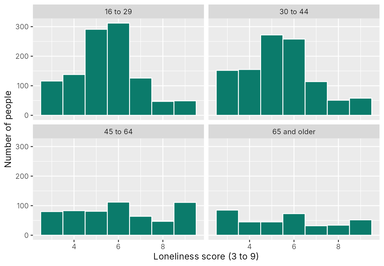
facet_wrap(~ age_group) (n = 3,083). The panels share both axes.The shared vertical axis shows both the shape and the size of each group. The two younger groups, with more than 1,000 people each, have tall bars at 5 and 6. The two older groups have shorter, flatter histograms with more people at both ends of the scale, and they hold most of the ceiling pile-up seen in Section 2: in the 45 to 64 group, 111 people scored 9, as many as scored 6 (112), and in the 65 and older group the most common score is 3, the lowest possible (85 people). The older groups are therefore more divided, with more people at the least lonely and the most lonely ends of the scale. If the groups' shapes matter more than their sizes, facet_wrap(~ age_group, scales = "free_y") gives each panel its own vertical axis, at the cost of making heights incomparable across panels.
facet_grid(gender ~ age_group) takes two variables, the first for the rows and the second for the columns, and draws one panel for every combination. Figure 6.17 shows social support against loneliness, with a straight line in each panel.
The lines slope downward in all twelve panels, so higher support goes with lower loneliness in every combination of gender and age group. The lines look steeper in the two older age groups: within the age groups as a whole, the slopes are about −0.40 and −0.54 points of loneliness per point of support in the two younger groups and about −0.76 and −0.84 in the two older groups. The table of counts printed in Activity 6.3 is the necessary companion to the grid. The non-binary panels hold between 6 and 26 people, so their lines and bands are very uncertain, and any difference they appear to show would need a much larger sample to assess. An exploratory figure should show small groups, and the text should say how small they are.
Table 6.6 gives these counts, the number of people behind each panel of Figure 6.17, as table(brief$gender, brief$age_group) prints them in Activity 6.3.
Table 6.6. Number of people in each panel of Figure 6.17, by gender and age group.
| Gender | 16 to 29 | 30 to 44 | 45 to 64 | 65 and older |
|---|---|---|---|---|
| Woman | 490 | 477 | 362 | 251 |
| Man | 564 | 557 | 204 | 109 |
| Non-binary | 25 | 26 | 12 | 6 |
Facets are one of the two ways of showing groups that Section 1 compared. The other is to map a variable to colour (for points and lines) or fill (for bars and boxes), which shows the groups within one panel. Colour lets the reader compare groups directly on the same axes, and it works well for two or three groups. Facets give each group its own panel, and they work better when there are many groups, when points overlap heavily, or when one group is much smaller than the others and would be hidden. The two can also be combined, with colour for one grouping variable and facets for another, as in the code read in Table 6.5. Once colour carries information, the colours themselves need care.
5.9 Colour-Blind-Safe Palettes, Themes and Saving a Figure
5.9.1 Palettes and Themes
A palette has to work for every reader. About 8% of men and 0.5% of women of northern European ancestry have some form of red-green colour-vision deficiency, so a palette that relies on telling red from green fails a sizeable part of any audience. The Okabe-Ito palette (Okabe & Ito, 2008) is a set of eight colours chosen to remain distinguishable for people with the common forms of colour-vision deficiency. Its first three colours after black, orange (#E69F00), sky blue (#56B4E9) and bluish green (#009E73), are used below with scale_fill_manual(). The viridis palettes, available in ggplot2 as scale_fill_viridis_d() for categories, are another safe choice, and they also remain readable when printed in greyscale. When a figure may be printed in black and white, or when readers may not separate even these colours, a second cue makes the groups distinguishable without colour: different point shapes (shape = group inside aes()), different line types (linetype = group), or one panel per group. Figure 6.18 maps fill to gender in boxplots of loneliness by age group, with the three Okabe-Ito colours and a minimal theme.
theme_minimal(base_size = 12) (n = 3,083).The theme controls the appearance of everything except the data. The default theme, theme_grey(), uses a grey panel with white grid lines. theme_minimal() removes the grey panel, theme_bw() adds a black border, and theme_classic() keeps only the axis lines. The argument base_size sets the size of all text in points, and 11 or 12 suits most journal figures. Labels are set with labs(), which also names the legend through the aesthetic it describes, as in fill = "Gender".
A colour-blind-safe palette with a second cue, and a plain theme with readable text, make a figure usable by every reader on screen. The last step is to save it to a file at the size at which it will be printed or shown.
5.9.2 Saving a Figure with ggsave()
The function ggsave() writes a ggplot2 plot to a file. Its first argument is the file name, and the extension sets the format: .png for most uses, .pdf or .svg for figures that must stay sharp at any size, and .tiff when a journal asks for it. The second argument is the plot object, here p, and without it ggsave() saves the last plot shown. The arguments width and height are in inches by default, and dpi sets the resolution, with 300 dots per inch the usual requirement for print. The size of the file in pixels is the width and the height multiplied by the dpi, and question 3 of Activity 6.3 has R work it out for the saved figure. Text size is relative to the physical size of the figure. By this we mean that base_size sets the text size in points for the figure at the width and height at which it is saved, and the text keeps that size only when the figure is shown at that size. If the figure is later shrunk to fit a much narrower space, such as a column of a page, everything in it shrinks by the same proportion, including the text. A plot saved at a large width with a small base_size will therefore have text that is too small when the figure is shrunk to fit a page, which is why a figure is best saved at the size at which it will be used.
Activity 6.3 practises the whole section. It draws every plot, from the histogram in Figure 6.12 to the coloured boxplots in Figure 6.18, prints the group means behind the geom_col() chart and the counts in Table 6.6, and saves the last plot with ggsave(). Download the code and run it along with the text version below, reading each layer as Table 6.5 does; the questions ask you to say in plain words what the layers do, to read the lines, bands and panel sizes, and to make the figure readable in black and white.
Text version of the activity: the code of the run-along script, its console output and notes on reading it.
brief <- read.csv("https://heal-learn.ca/r-activities/data/cscs_brief.csv")   # course data, read from the website
brief$age_group <- factor(brief$age_group,
  levels = c("16 to 29", "30 to 44", "45 to 64", "65 and older"))
brief$gender <- factor(brief$gender, levels = c("Woman", "Man", "Non-binary"))
brief$mental_health <- factor(brief$mental_health,
  levels = c("Poor", "Fair", "Good", "Very good", "Excellent"))
nrow(brief)                      # one row per person
# install.packages("ggplot2")    # once per computer, if not yet installed
library(ggplot2)The briefing file is the one built in Section 2: 3,083 people with no missing value on the nine briefing variables. A file read with read.csv() stores categories as text, so factor() with levels restores their order. ggplot2 is installed once on each computer with install.packages("ggplot2") and loaded with library(ggplot2) in every new session; if R reports could not find function "ggplot", run library(ggplot2) again.
ggplot(brief, aes(x = loneliness)) +               # data and mapping
  geom_histogram(binwidth = 1,                     # one bar per score
                 fill = "#0B7B6B", colour = "white") +   # set, not mapped
  labs(title = "Loneliness scores",
       x = "Loneliness score (3 to 9)", y = "Number of people")
ggplot(brief, aes(x = mental_health)) +
  geom_bar() +                                     # counts the rows
  labs(x = "Self-rated mental health", y = "Number of people")
means <- aggregate(loneliness ~ age_group, data = brief, FUN = mean)
means                                              # one row per age group
ggplot(means, aes(x = age_group, y = loneliness)) +
  geom_col() +                                     # draws the values given
  labs(x = "Age group", y = "Mean loneliness score")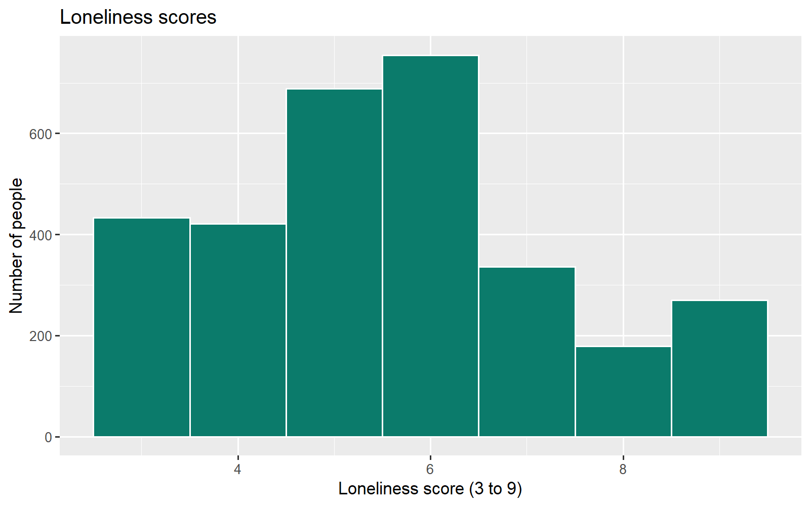
Each plot starts with the data and the aesthetic mapping, and every further part is added with a plus sign at the end of the line before it. The fill and outline colours of the histogram are set outside aes(), so every bar is teal with a white outline; a fixed colour written inside aes() would be treated as a variable, drawn in a default colour and given a legend. geom_bar() counts the rows in each category (Very good is the most common rating), while geom_col() draws the four means computed by aggregate(), from 5.39 to 6.01. Used on the table of means, geom_bar() stops with the error stat_count() must only have an x or y aesthetic, and with only x mapped it would draw four bars of height 1.
set.seed(2021)                                     # the same jitter every time
ggplot(brief, aes(x = age_group, y = loneliness)) +
  geom_boxplot(outlier.shape = NA) +               # no separate outlier dots
  geom_jitter(width = 0.2, height = 0.2, alpha = 0.1) +   # every person
  labs(x = "Age group", y = "Loneliness score (3 to 9)")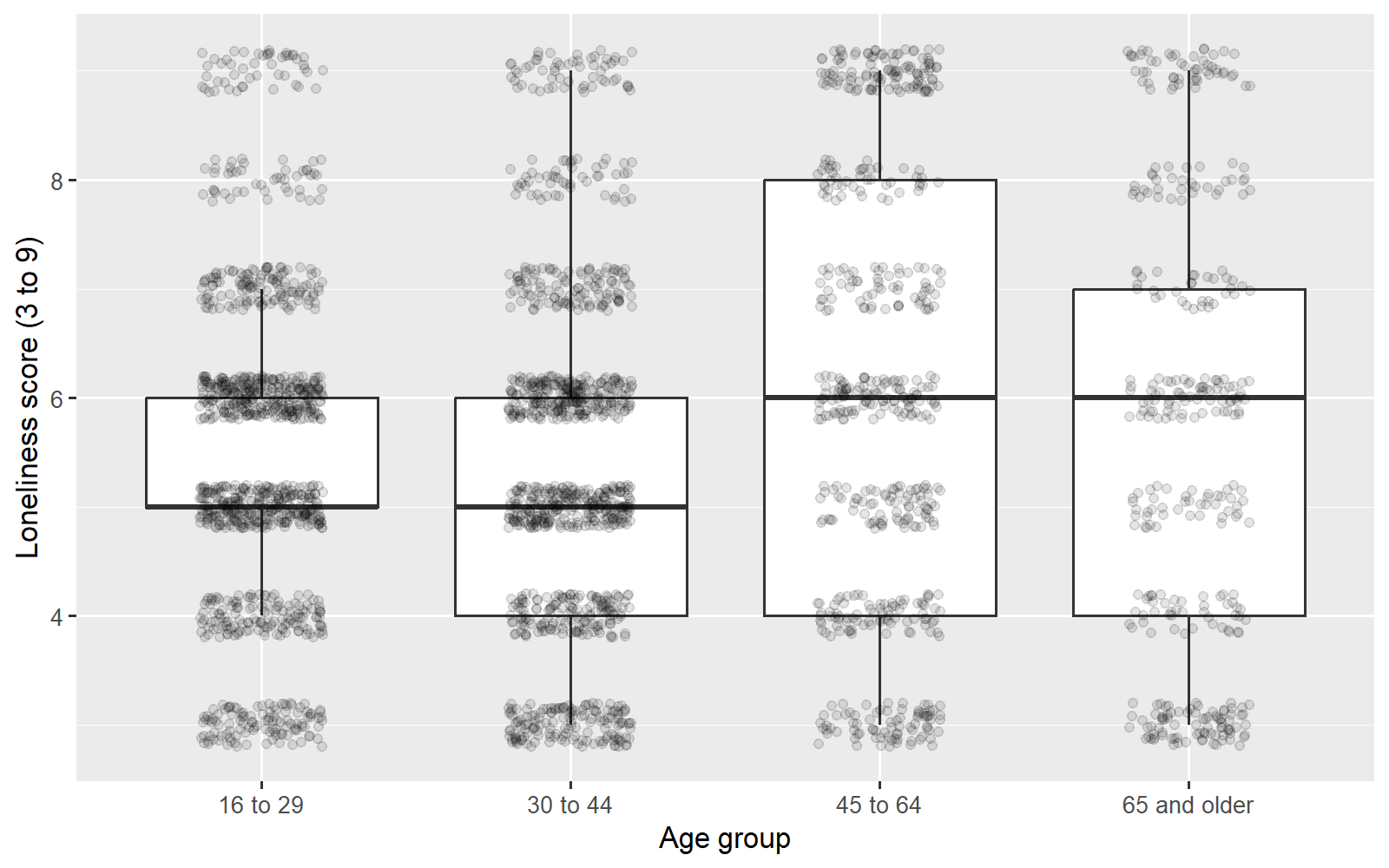
The boxplot layer draws the median, the quartiles and the whiskers for each age group, and outlier.shape = NA stops it from drawing outlying people a second time, because geom_jitter() draws every person. width and height set how far each point may be nudged, and alpha = 0.1 makes the points nearly transparent; set.seed(2021) makes the jitter the same every time the code runs. The medians are 5, 5, 6 and 6, every group spans the whole scale from 3 to 9, and the 65 and older group (366 people) is the smallest.
set.seed(2021)
ggplot(brief, aes(x = age, y = loneliness)) +
  geom_jitter(height = 0.2, alpha = 0.1) +
  geom_smooth(method = "loess") +                  # a curve that can bend
  labs(x = "Age (years)", y = "Loneliness score (3 to 9)")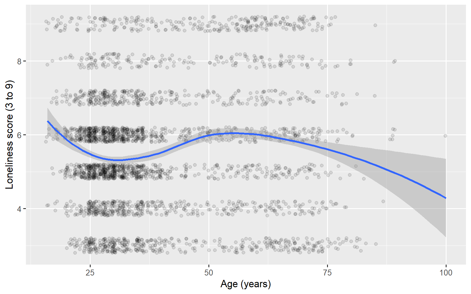
The message reports the formula that geom_smooth() used and is not an error. The loess curve is about 6.4 at age 16, dips to about 5.3 around age 30, rises to about 6 between 50 and 60 and falls after 70. The grey band is its 95% confidence band; it widens at both ends, where only 48 people are under 20 and 29 are 80 or older, so the ends deserve the least trust.
ggplot(brief, aes(x = loneliness)) +
  geom_histogram(binwidth = 1, fill = "#0B7B6B", colour = "white") +
  facet_wrap(~ age_group) +                        # one panel per age group
  labs(x = "Loneliness score (3 to 9)", y = "Number of people")
set.seed(2021)
ggplot(brief, aes(x = support, y = loneliness)) +
  geom_jitter(height = 0.2, alpha = 0.2) +
  geom_smooth(method = "lm") +                     # a straight line per panel
  facet_grid(gender ~ age_group) +                 # rows: gender; columns: age
  labs(x = "Social support (1 to 7)", y = "Loneliness score (3 to 9)")
table(brief$gender, brief$age_group)               # people in each panel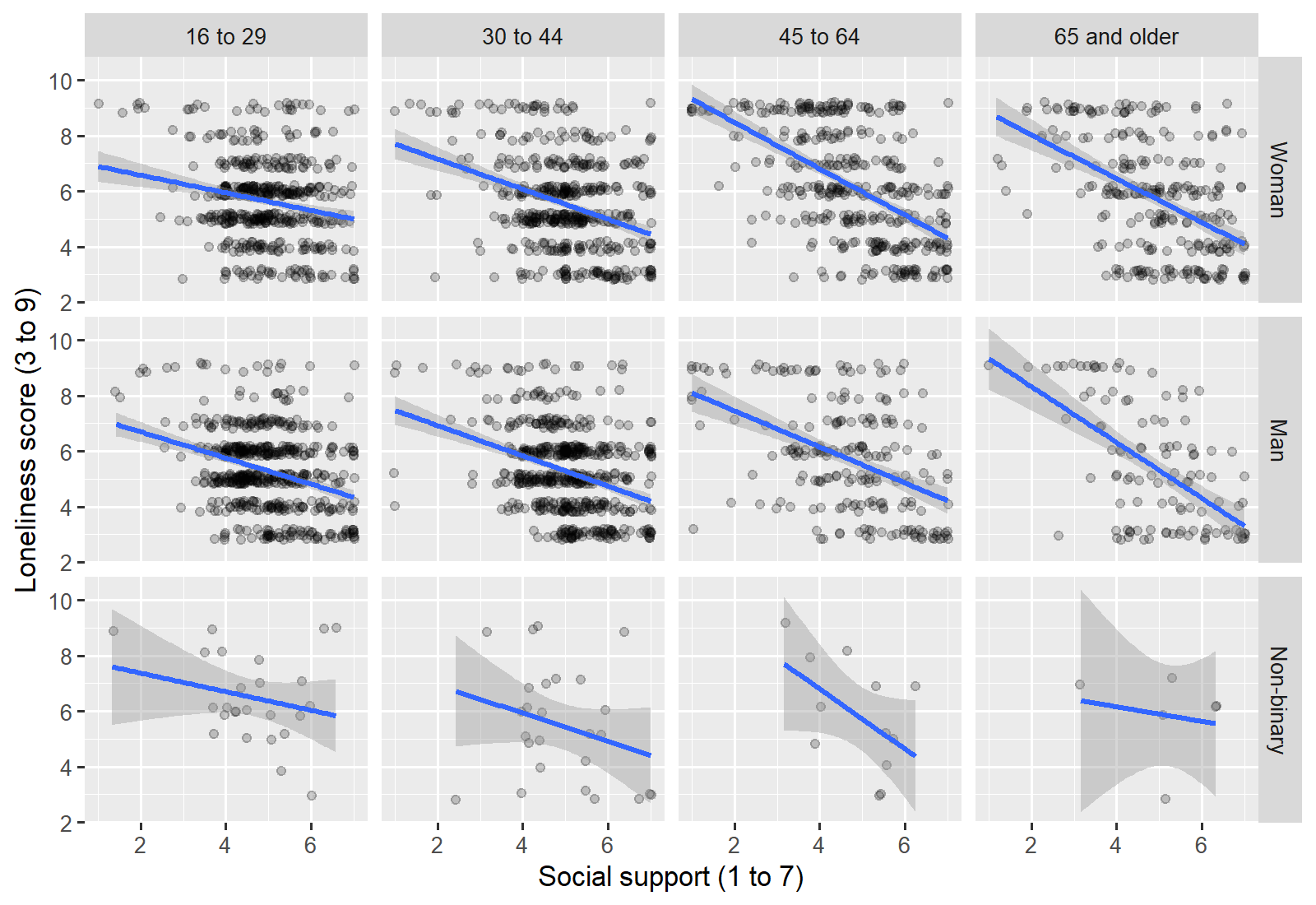
facet_wrap(~ age_group) draws one histogram per age group on shared axes, and facet_grid(gender ~ age_group) draws one panel for each combination of gender (rows) and age group (columns), here with a straight least-squares line (method = "lm") in each panel. The table gives the number of people behind each panel: the non-binary panels hold only 25, 26, 12 and 6 people.
p <- ggplot(brief, aes(x = age_group, y = loneliness, fill = gender)) +
  geom_boxplot() +
  scale_fill_manual(values = c("#E69F00", "#56B4E9", "#009E73")) +   # Okabe-Ito
  labs(x = "Age group", y = "Loneliness score (3 to 9)", fill = "Gender") +
  theme_minimal(base_size = 12)                    # a plain theme
p                                                  # show the plot
ggsave("loneliness_age_gender.png", p, width = 7, height = 4.5, dpi = 300)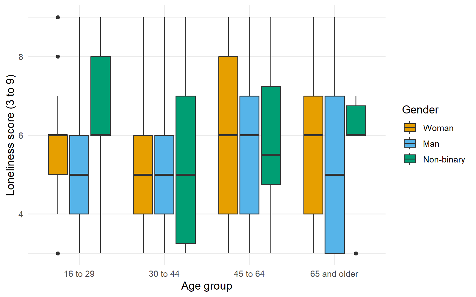
Storing the plot as p lets the same object be shown on screen and saved. The three fill colours are from the Okabe-Ito palette. ggsave() writes loneliness_age_gender.png, 7 by 4.5 inches at 300 dots per inch (2,100 by 1,350 pixels), and prints nothing.
R Reflect on what you just ran
Answer each question from your own output, as on the final exam: say in plain words what each layer does for the figure, read the lines, bands and panel sizes, and make the figure readable for every reader.
1. Say in plain words what geom_boxplot(outlier.shape = NA) and geom_jitter(width = 0.2, height = 0.2, alpha = 0.1) do for this figure, and why the points are jittered and drawn partly transparent. The bar chart drawn with geom_col() summarizes each age group by its mean: name two things that display hides and this figure shows.
geom_boxplot(outlier.shape = NA), draws a box for each age group, with the median, the quartiles and the whiskers, and leaves out separate outlier dots because the jittered points already show everyone. The jitter layer, geom_jitter(width = 0.2, height = 0.2, alpha = 0.1), draws one point per person, shifted a little at random sideways and up or down, so that the many people who share a score do not sit on top of one another; the transparency makes crowded areas darker, and the shift changes only where the points are drawn, not the data. Compared with four means between 5.39 and 6.01, the figure shows the spread within each group: every age group has scores across the whole range from 3 to 9, and the box for 45 to 64 runs from 4 to 8. It also shows the size of each group, with far fewer dots for the 366 people aged 65 and older than for the 1,079 aged 16 to 29, and it shows the medians of 5, 5, 6 and 6.2. Describe what the lines in the facet_grid(gender ~ age_group) figure show about social support and loneliness, and say what the grey band around each line shows. If the briefing shows this grid, what should its text say about the size of the non-binary panels, and why? Use the table of counts.
3. Run your own code: at the end of your script, type p + aes(linetype = gender) + labs(linetype = "Gender") and c(width = 7, height = 4.5) * 300 and run them. Some readers of the working group's report have colour-vision deficiency, and the report may be printed in black and white. Explain why the script uses the three Okabe-Ito colours rather than the default colours, and what your first line adds for a black-and-white printout. Then state what the width, height and dpi arguments of ggsave() control, and what the output of your second line tells you about the saved file.
ggsave(), width and height set the physical size of the figure in inches (7 by 4.5), and dpi sets the resolution in dots per inch (300, the usual print standard). Your second line multiplies the width and the height by the resolution, and its output shows that the saved file is 2,100 pixels wide and 1,350 pixels high, enough for a sharp print at 7 by 4.5 inches.Your plots and output reproduce Figures 6.12 to 6.18 and Table 6.6, so each reading in this section can be checked against your own screen. If any step felt fast, the narrated walkthrough introduced in Section 2 builds the same plots layer by layer; the card below links to it again.
Narrated R walkthrough: Data Visualization in Base R and ggplot2
The walkthrough builds the ggplot2 plots in this section layer by layer, so that the effect of each line of code can be seen before the next is added.
Open the walkthroughThis section has described the grammar on which ggplot2 is built and used it to read a figure's code, to draw the briefing plots for one variable, for a numeric variable across groups and for two numeric variables, to compare groups with facets and colour, and to make and save a figure that every reader can use. The key takeaways below summarize these steps, the knowledge check reviews them, and Section 4 adds displays for many variables and combines the briefing plots into one figure.
Key Takeaways
- 5.4 ggplot2 builds every plot from the same few parts, so once you know them you can read almost any figure's code. The data are a data frame with one row per person; aesthetics, written inside
aes(), map variables to visual properties such asx,y,colourorfill; and geoms are the marks that draw the data, such as boxes, points or lines. Scales, facets and a theme have sensible defaults and are added as further layers when needed, each joined to the plot with a plus sign at the end of the line before it. To explain code in plain words, ask what each line adds to the picture, as Table 6.5 does:colour = gendergives each gender its own colour and adds a legend, andfacet_wrap(~ age_group)makes one panel per age group on the same axes. Watch for the classic slip of putting a fixed colour insideaes():aes(colour = "blue")treats "blue" as if it were a variable, whereas a fixed colour belongs outside, as ingeom_point(colour = "blue"). - 5.5 One template,
ggplot(data, aes(...)) + geom_...() + labs(...) + theme_...(), draws every display in this section, and only the mapping and the geom change.geom_histogram(binwidth = 1)gives a histogram with one bar per whole score,geom_bar()a bar chart of counts,geom_boxplot(outlier.shape = NA)withgeom_jitter(width = 0.2, height = 0.2, alpha = 0.1)a boxplot with every person shown as a faint dot, andgeom_jitter()withgeom_smooth()a scatterplot with a smoother. Because each geom is a layer, several can be stacked on the same axes;outlier.shape = NAsimply stops the boxplot from drawing outlying people a second time when the jittered points already show everyone. If R reportscould not find function "ggplot", runlibrary(ggplot2), and keep each plus sign at the end of a line, never at the start of the next. When a question shows a block of ggplot2 code, be ready to say which display it produces and what each geom adds to it. - 5.6
geom_bar()andgeom_col()both draw bars, but they get their heights in different ways.geom_bar()counts the rows in each category, so it needs only anxaesthetic and suits raw data with one row per person, such as the number of people giving each mental health rating.geom_col()draws heights that are already in the data, so it needs bothxandyand suits a small summary table, such as the four age-group means computed withaggregate(). The tell-tale mistake is usinggeom_bar()on a summary table, which gives every bar a height of 1 because each group appears in only one row. Before choosing, ask whether each row is a person to be counted or a group whose value has already been computed, and remember that a chart of group means is the "means without spread" display from Section 1, so for the briefing, boxplots with points are better. - 5.7
geom_smooth()adds a line that follows the average ofyacross the values ofx:method = "loess"draws a loess smoother, which can bend, andmethod = "lm"draws a straight least-squares line. The grey band around the line is its 95% confidence band, which shows how uncertain the position of the average is; it is not the spread of individual people, most of whom lie outside it, andse = FALSEdraws the line without it. The line deserves the least trust where few people sit behind it, usually at the ends, and you can spot this because the band widens there (in Figure 6.15, only 48 respondents are under 20 and 29 are 80 or older). To describe such a plot, say the direction and form of the pattern in plain words (loneliness is highest among the youngest, dips around age 30, rises to about 6 in the fifties and falls after 70), note where the band is wide, and remember that a smoother describes the data and gives no reason for the pattern. The message`geom_smooth()` using formula = 'y ~ x'is only a note, not an error. - 5.8
facet_wrap(~ group)draws the same plot once for each level of one grouping variable and wraps the panels into a grid, andfacet_grid(rows ~ columns)uses two variables, one for the rows and one for the columns, as infacet_grid(gender ~ age_group). The panels share their axes by default, so heights and slopes can be compared directly;scales = "free_y"gives each panel its own vertical axis, at the cost of that comparison. Use colour for two or three groups that overlap little, and facets for many groups, heavily overlapping points or groups of very different sizes. Always check how many people sit behind each panel, for example withtable(brief$gender, brief$age_group): the non-binary panels in Figure 6.17 hold only 6 to 26 people, so their lines and bands are very uncertain. Show small panels rather than hiding them, but state how many people they hold and avoid drawing conclusions from them. - 5.9 About 8% of men and 0.5% of women of northern European ancestry have some form of red-green colour-vision deficiency, so a palette that depends on telling red from green fails part of any audience. Use a colour-blind-safe palette such as Okabe-Ito (for example
scale_fill_manual(values = c("#E69F00", "#56B4E9", "#009E73"))) or viridis (scale_fill_viridis_d()), and if the figure may be printed in black and white, add a second cue that does not rely on colour: point shapes (shape = group), line types (linetype = group) or one panel per group. A theme such astheme_minimal(base_size = 12)sets the background and the text size without changing the data. Save the finished figure withggsave("file.png", p, width = 7, height = 4.5, dpi = 300): the width and height are in inches, and 300 dpi is the usual print standard, giving a file of 2,100 by 1,350 pixels. When asked how to help readers with colour-vision deficiency, a full answer names both a safe palette and a second cue.
1. A colleague drew a figure of waiting times at three walk-in clinics with the code below. In plain words, what do the second and third lines do for the figure?
ggplot(dat, aes(x = clinic, y = wait)) +
  geom_boxplot(outlier.shape = NA) +
  geom_jitter(width = 0.2, height = 0, alpha = 0.2) +
  labs(x = "Walk-in clinic", y = "Waiting time (minutes)") +
  theme_minimal()
geom_boxplot() draws the median, quartiles and whiskers for each clinic, and outlier.shape = NA only stops it drawing its own points beyond the whiskers, because geom_jitter() already draws every patient; in that layer width = 0.2 nudges each point sideways, height = 0 leaves each waiting time exactly where it is, and alpha = 0.2 sets the opacity to 20%, so crowded waits look darker. The option about removing patients is tempting, but outlier.shape = NA hides duplicate marks and removes nobody from the data; the jitter layer still shows the patients with the longest waits. (Section 3, 5.4.3 Reading a Figure's Code in Plain Words, Table 6.5, and 5.5.2 A Numeric Variable Across Groups; Objectives 5.4 and 5.5)2. A colleague computed a small data frame, rates, with one row per health region and a column pct_vacc that holds the percentage of adults vaccinated against influenza. The code ggplot(rates, aes(x = region)) + geom_bar() draws a bar of height 1 for every region. Why, and what is the fix?
geom_bar() counts the rows in each category, so the fix is to map pct_vacc to y and use geom_col(). The information needed is the shape of the data frame (one row per region, with the values already computed) and what each geom does. geom_bar() needs only x and counts the rows in each category, which suits a file with one row per person; here each region appears in one row, so every count is 1. geom_col() draws bars whose heights are supplied in the data, as in the bar chart of mean loneliness by age group built from aggregate(). The histogram option is tempting because the percentages are numeric, but a histogram bins one numeric variable along a number line and would not draw one bar per region. (Section 3, 5.6 Counting Rows or Drawing Values: geom_bar() and geom_col(), Figure 6.13; Objective 5.6)3. A scatterplot of self-reported daily steps against age for 1,900 adults has jittered, see-through points and a curve from geom_smooth(method = "loess"). The curve is flat at about 7,500 steps from age 20 to 50, falls to about 5,000 steps at age 75, and turns upward after 85. The grey band is narrow between ages 25 and 65 and very wide above 80, where 14 of the 1,900 adults are. Which statement is correct?
4. A figure shows body mass index against age with a straight line in each panel of facet_wrap(~ region). The table gives the number of adults in each panel. In region F the line slopes downward, while the lines in the other five panels slope upward. What should the briefing say about region F?
| Region | A | B | C | D | E | F |
|---|---|---|---|---|---|---|
| Adults in the panel | 410 | 385 | 352 | 298 | 41 | 9 |
5. A figure for a printed report shows systolic blood pressure against age, with one line for women (red) and one for men (green). Some readers have red-green colour-vision deficiency, and the report will be printed in black and white. Which change lets every reader tell the two lines apart?
dpi set in ggsave() controls the sharpness of the file, not which colours readers can separate. (Section 3, 5.9 Colour-Blind-Safe Palettes, Themes and Saving a Figure; Objective 5.9)6. A health unit surveyed 1,350 adults in five regions about recreational screen time and sleep. Four regions hold between 290 and 360 respondents each, and the North region holds 40. The figure was drawn with the code below. In the four large regions, the curves for both sexes fall from about 8.0 hours of sleep at 1 hour of screen time to about 6.5 hours at 6 hours, and the grey bands widen beyond 6 hours, where only 30 respondents are found. In the North panel the two curves cross. Which reading of the code and the figure is correct?
ggplot(svy, aes(x = screen_hrs, y = sleep_hrs, colour = sex)) +
  geom_jitter(width = 0.2, height = 0.2, alpha = 0.2) +
  geom_smooth(method = "loess") +
  facet_wrap(~ region) +
  labs(x = "Recreational screen time (hours per day)",
       y = "Sleep (hours per night)", colour = "Sex") +
  theme_minimal()
colour = sex maps sex to colour, so each sex gets its own colour, legend entry and curve; geom_jitter() spreads out people who gave the same answers; geom_smooth(method = "loess") draws a curve of average sleep that can bend, with a grey 95% confidence band for that average; and facet_wrap(~ region) draws one panel per region on the same axes. In the large regions, adults with more screen time tend to sleep less, which describes the data and does not show that screen time shortens sleep. The bands widen where few people are, beyond 6 hours of screen time, and the two curves in the North panel rest on only 40 people between them, so the crossing could easily be chance; the panel is shown, its size is stated, and no conclusion is drawn from it. The first option is the common misreading of the band, which shows uncertainty about the average, not the spread of individual people. (Section 3, 5.4.3 Reading a Figure's Code in Plain Words, 5.7 Reading a Scatterplot with a Smoother and 5.8 Comparing Groups with Facets; Objectives 5.4, 5.7 and 5.8)Many Variables and Combined Figures
A correlation matrix drawn as colours
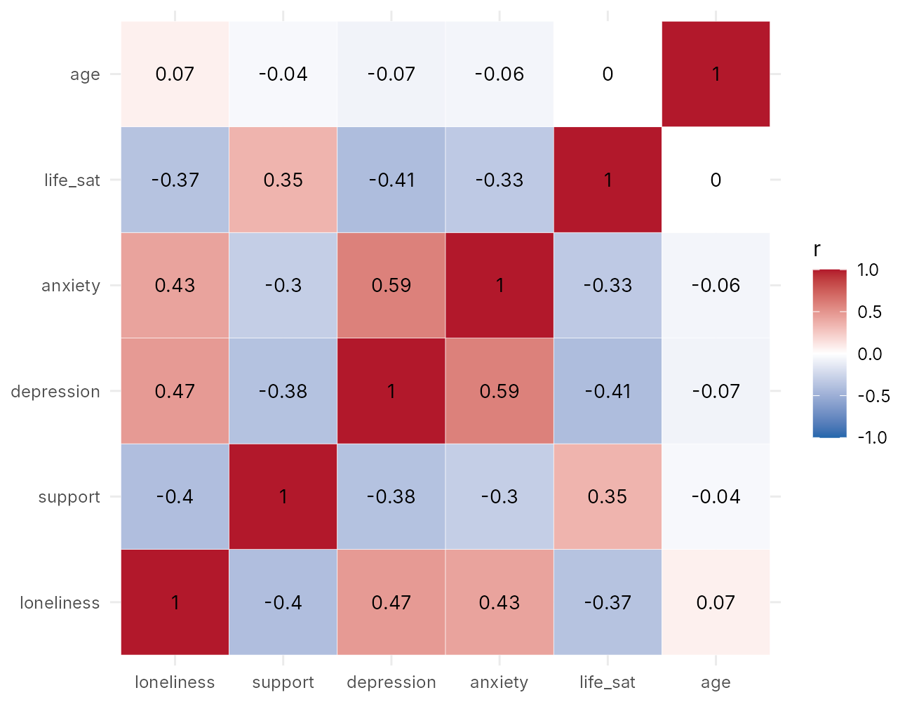
A relationship and two distributions in one display
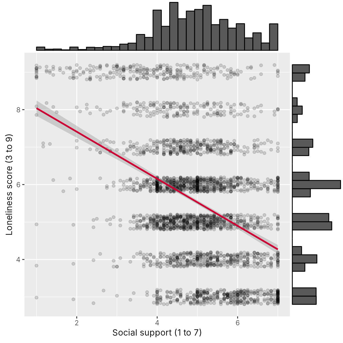
ggMarginal(p_scatter, type = "histogram").The briefing as one figure
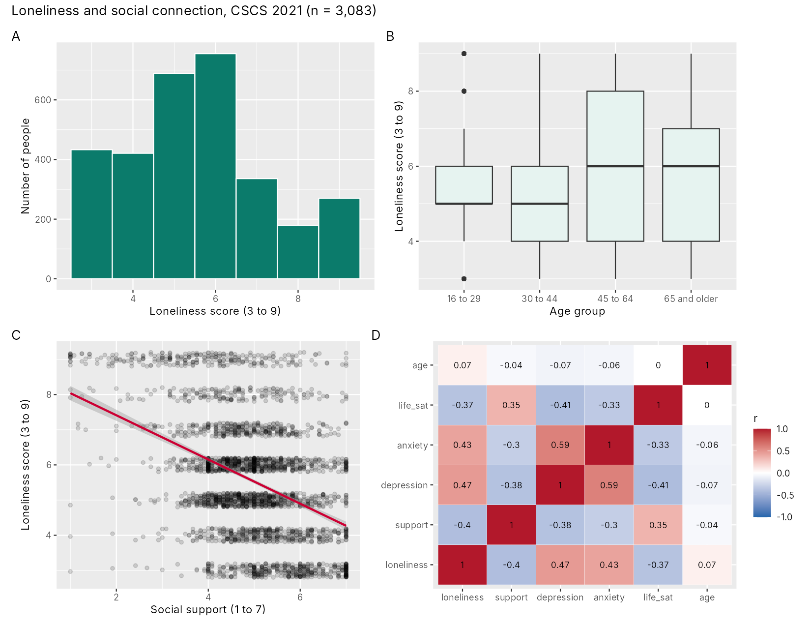
(p_hist + p_box) / (p_scatter + p_heat) + plot_annotation(tag_levels = "A")Overview
The working group's third question asks how loneliness goes together with social support and mental health, which involves several variables at once. One scatterplot per pair would answer it slowly, because six variables have fifteen pairs. This section shows how to summarize many pairs in one display with a correlation matrix and a heatmap, when Spearman's rank correlation is the better summary, and what such a summary cannot show. It then adds marginal histograms to a scatterplot, combines the briefing plots into one multi-panel figure checked against the conventions of a publication figure, and writes the caption that lets the figure stand on its own. The finished figure is the kind of exploratory figure that a research paper based on survey data often includes.
Learning Objectives
- 6.1 Compute a correlation matrix with
cor(), display it as a heatmap in ggplot2, and describe a correlation in words by its direction and strength. - 6.2 Explain when Spearman's rank correlation is preferred to Pearson's r.
- 6.3 Explain why a correlation heatmap shows association and cannot identify causes, curved relationships or the shape of the data.
- 6.4 Build and read a scatterplot with marginal histograms using
ggExtra::ggMarginal(). - 7.1 Combine several ggplot2 plots into one labelled figure with the patchwork package, save it with
ggsave(), and check it against the conventions of a publication figure. - 7.2 Write a caption that states what the figure shows, so that it stands on its own, and keep interpretation for the results text.
6.1 Correlation Matrices and Heatmaps
6.1.1 The Correlation Matrix
The Pearson correlation coefficient, written r, measures how closely two numeric variables follow a straight line. By this we mean that it describes how tightly the points of a scatterplot cluster around a straight line, and whether that line slopes up or down. It ranges from −1 (all points on a line sloping downward) through 0 (no straight-line relationship) to +1 (all points on a line sloping upward). Its sign gives the direction: a positive r means that people with higher values on one variable tend to have higher values on the other, and a negative r means that higher values on one tend to go with lower values on the other. Its size, ignoring the sign, gives the strength: the closer r is to −1 or +1, the more tightly the points cluster around a line, and the closer it is to 0, the more loosely they are scattered. Cohen (1988) suggested that values of about 0.1, 0.3 and 0.5 be called small, medium and large in the behavioural sciences, and these labels are a rough guide only, since what counts as a strong association depends on the field and the question.
The function cor(), given a data frame of numeric columns, returns a correlation matrix with one row and one column per variable. Each cell holds the correlation between its row variable and its column variable. The diagonal holds the correlation of each variable with itself, which is always 1, and the matrix is symmetric, so the values above the diagonal repeat those below it. Six variables give 36 cells and 15 distinct correlations.
Table 6.7 gives the correlation matrix for the six numeric briefing variables, as cor() prints it in Activity 6.4.
Table 6.7. Pearson correlations among the six numeric variables in the briefing file (n = 3,083).
| loneliness | support | depression | anxiety | life_sat | age | |
|---|---|---|---|---|---|---|
| loneliness | 1.00 | −0.40 | 0.47 | 0.43 | −0.37 | 0.07 |
| support | −0.40 | 1.00 | −0.38 | −0.30 | 0.35 | −0.04 |
| depression | 0.47 | −0.38 | 1.00 | 0.59 | −0.41 | −0.07 |
| anxiety | 0.43 | −0.30 | 0.59 | 1.00 | −0.33 | −0.06 |
| life_sat | −0.37 | 0.35 | −0.41 | −0.33 | 1.00 | 0.00 |
| age | 0.07 | −0.04 | −0.07 | −0.06 | 0.00 | 1.00 |
In the briefing file, loneliness has moderate positive correlations with depressive symptoms (0.47) and anxiety symptoms (0.43), and moderate negative correlations with social support (−0.40) and life satisfaction (−0.37). Its correlation with age is close to zero (0.07). The strongest correlation in the matrix is between depressive and anxiety symptoms (0.59), two measures that often move together. To find the strongest correlation with one variable, read along its row, skip the 1 on the diagonal, and compare the sizes whatever their sign.
A correlation is put into words about people, not units. The value of −0.40 for social support and loneliness means that people with more social support tend to report less loneliness, a moderate negative association. It has no units and it is not a slope. This is because r is calculated after each variable has been put on a common standardized scale, so it measures how consistently the two variables move together, not how much one changes when the other changes. It therefore does not mean that loneliness falls by 0.40 points for each extra point of support (that would be a regression slope, which depends on the units of both variables), and it is not a percentage, either of the variation in loneliness or of the people in the file. One practical point also applies to cor(): it returns NA for any pair with a missing value unless told how to handle them, for example with use = "complete.obs". The briefing file has no missing values, so this does not arise here.
A matrix of 36 numbers is slow to read, and the same matrix can be drawn in colour.
6.1.2 Drawing the Matrix as a Heatmap
A correlation heatmap draws each cell of the matrix as a coloured square, so that the pattern can be seen at a glance. Drawing it in ggplot2 takes two steps. The matrix is first turned into a long data frame with one row per pair. By this we mean that the square table, in which each correlation sits where a row meets a column, is rearranged into a list in which each correlation has its own row, with one column naming the first variable, one naming the second and one holding the value. ggplot2 needs the data in this form because each aesthetic is mapped to a column: a square can be placed at its horizontal and vertical position and coloured by its value only if those three pieces of information are stored as three columns. In the code, as.table() treats the matrix as a table, and as.data.frame() turns that table into three columns, here renamed var1, var2 and r. Then geom_tile() draws one square per row, with var1 mapped to x, var2 to y and r to fill, and geom_text() prints the value on each square. Figure 6.19 shows the heatmap for the six briefing variables.
The colour scale is a diverging scale, set with scale_fill_gradient2(): blue for negative values, white at zero and red for positive values, with limits = c(-1, 1) so that the colours keep the same meaning in any heatmap. A diverging scale is one that runs outward in two directions from a neutral middle colour. It suits correlations because zero is a meaningful midpoint: it separates negative associations from positive ones. As a result, the hue of a square shows the direction of the correlation at a glance, and the depth of the colour shows its strength, with pale squares near zero and deep colours near −1 or +1. Blue and red remain distinguishable for people with red-green colour-vision deficiency, which a red-to-green scale would not.
The heatmap shows a clear structure. Loneliness, depression and anxiety form a block of positive correlations, and each of the three is negatively correlated with social support and life satisfaction, which are positively correlated with each other (0.35). Age is close to white in every square. For the briefing, this panel gives the working group an overview of the third question in one picture.
Every square in the heatmap is a Pearson correlation, which is not always the best single number for the kinds of scores a survey produces.
6.2 When Spearman's Rank Correlation Is Preferred
Pearson's r assumes numeric variables and is sensitive to outliers and to skew, because it is calculated from the actual values, so a few very large or very small values can pull it up or down. For ordinal scores or skewed variables, Spearman's rank correlation, computed with cor(..., method = "spearman"), uses the ranks of the values instead. By this we mean that each variable is first replaced by the positions of its values when they are sorted from smallest to largest (1 for the smallest, 2 for the next, and so on, with tied values sharing the average of their positions), and the correlation is then calculated on those ranks. Because a rank records only order, an extreme value simply receives the highest or lowest rank, however far it lies from the others, so Spearman's correlation is less affected by extreme values. In addition, it measures whether one variable tends to rise as the other rises, whether or not the rise follows a straight line, which suits ordered ratings whose categories are not evenly spaced. For loneliness and social support, Spearman's correlation is −0.36, close to the Pearson value of −0.40. When the two values are similar, the Pearson value is not being driven by a few extreme values; when they differ noticeably, the shape of the data (skew, a pile-up at a top-coded value, or a relationship that rises and then levels off) deserves a scatterplot before either number is reported.
The cue for Spearman's correlation is usually in the description of the variable: an ordered rating, a strongly skewed count, or a long tail of extreme or piled-up values. Activity 6.4 prints both coefficients for loneliness and social support, so the comparison can be checked on your own output. Whichever coefficient is used, it remains one number per pair, and one number per pair has limits.
6.3 What a Correlation Heatmap Cannot Show
A correlation heatmap shows the strength and direction of straight-line association between each pair of variables. Three common readings go beyond what it shows: that a correlation identifies a cause, that a correlation near zero means there is no relationship, and that one number describes the data. Expand each panel of the accordion below to see why the heatmap cannot support each reading, with examples from the briefing.
The correlation of 0.47 between loneliness and depressive symptoms is consistent with several causal stories. Loneliness might increase depressive symptoms. Depression might lead people to withdraw from others and feel lonelier, which is reverse causation. Other factors, such as poor physical health, bereavement or low income, might increase both, which is confounding by a common cause. All three stories, and combinations of them, would produce the same square on the heatmap. The CSCS 2021 data were collected at one time point, so the order of events cannot be established from them. Separating these explanations requires study design, causal diagrams of the kind drawn in earlier courses, and models that adjust for confounders, and even then a cross-sectional survey supports causal claims only weakly. A heatmap is therefore a map of where to look, and the briefing should describe it as showing which measures go together.
Pearson's r measures how well a straight line describes the data. The correlation between age and loneliness is 0.07, yet the loess curve in Section 3 showed a clear pattern: loneliness dips around age 30, rises into the fifties and falls after 70. Rises and falls in different parts of the age range cancel out in a single straight-line summary. By this we mean that a straight line fitted across the whole age range must choose one overall direction, and where loneliness rises with age in some parts of the range and falls in others, those stretches pull the line in opposite directions and leave it almost flat. A near-white square means only that no straight line fits well, and a scatterplot is needed to see whether a curve does.
Anscombe's quartet in Section 1 showed four datasets with the same correlation of 0.82 and completely different shapes, including a curve, an outlier and a relationship created by a single point. A heatmap reduces each pair to one number, so it hides outliers, clusters, floors and ceilings, and it says nothing about how many people contributed. Strong or surprising squares should be followed up with a scatterplot of that pair.
Each panel ends at the same place: a heatmap shows association only, and it points to the pairs of variables that deserve a closer look. One way to take that closer look is a scatterplot of one pair with the distribution of each variable along its margins.
6.4 Scatterplots with Marginal Histograms
A scatterplot shows how two variables go together, and a histogram shows how one variable is distributed. A scatterplot with marginal histograms shows both at once: the scatterplot sits in the middle, with a histogram of the horizontal variable along the top and a histogram of the vertical variable along the right side. The function ggMarginal() from the ggExtra package adds the margins to a finished ggplot2 scatterplot. Its argument type can be "histogram", "density" or "boxplot". Figure 6.20 shows loneliness against social support with a histogram of each variable along its margin.
The marginal histogram of social support shows a distribution skewed to the left: most people have scores between 4 and 6, and a long, thin tail runs toward low support. It also shows spikes at whole-number scores. In the briefing file, 170 people have a score of exactly 5, 136 exactly 4 and 117 exactly 7. The support score is the mean of twelve items, so a whole-number score is what a person who gives the same answer to every item receives, and a score of 7 requires the highest answer on all twelve. Such answers can reflect genuine views or a respondent moving quickly through the questions (sometimes called straight-lining), and the plot is a reason to look more closely before analyzing the score. The marginal histogram of loneliness shows the seven separate values of that score.
The object that ggMarginal() returns is a finished drawing, and it is not a ggplot2 object, so further layers cannot be added to it and patchwork cannot place it in a grid without extra steps. It can be saved with ggsave(). The combined briefing figure (Figure 6.21) therefore uses the scatterplot without its margins.
The marginal histograms add what the heatmap could not: the shape of each variable, here the spikes in the support score at whole-number values. With the displays for many variables in hand, the briefing plots can now be assembled into a single figure.
7.1 Combining Panels into a Publication Figure
7.1.1 Combining Panels with patchwork
A multi-panel figure lets a reader see several related displays together, with consistent styling and one caption. The patchwork package combines ggplot2 plots with arithmetic-like operators. A plus sign (+) or a vertical bar (|) places plots side by side, a forward slash (/) stacks them, and parentheses group them. The expression (p_hist + p_box) / (p_scatter + p_heat) therefore gives two plots in the top row and two in the bottom row. The function plot_annotation() adds a title, a subtitle or a caption to the whole figure, and its argument tag_levels = "A" labels the panels A, B, C and D in reading order, which the caption can then refer to. The function plot_layout() controls the number of columns, the relative widths and heights of panels, and whether legends are collected in one place. Figure 6.21 shows the draft briefing figure that this expression produces from the histogram, the boxplots, the scatterplot and the heatmap.
The figure is saved with ggsave("briefing_figure.png", figure, width = 11, height = 8.5, dpi = 300). A four-panel figure needs a larger size than a single plot, so that each panel keeps legible text, and 11 by 8.5 inches suits a full page turned sideways or a slide. When the figure is placed in a narrower space, such as one column of a journal, it is better to save it at that width and adjust the text size with base_size than to shrink a large image.
The draft in Figure 6.21 still shows R variable names in panel D, which is one of the things a check against the conventions of a publication figure catches.
7.1.2 Conventions of a Publication Figure
An exploratory figure in a manuscript has a different audience from the analyst's quick looks. Readers see it once, often without the text nearby, and they should be able to understand it without access to the code. Tufte (1983) argued that a graphic should spend its ink on the data and remove decoration that carries no information, which he called chartjunk. Table 6.8 lists the conventions most journals expect and checks the draft briefing figure against them; read down the third column to see which conventions the draft already meets and which it does not.
Table 6.8. Conventions of a publication figure, checked against the draft briefing figure (Figure 6.21).
| Convention | What it means | Draft briefing figure |
|---|---|---|
| Axis labels in words, with units or ranges | "Loneliness score (3 to 9)" in place of loneliness | Met in panels A to C |
| Plain labels for variables | "Life satisfaction" in place of life_sat | Not yet met in panel D, which shows R names |
| Panel letters | A, B, C and D, referred to in the caption | Met with tag_levels = "A" |
| Legends that name their scale | The fill legend in panel D is labelled r | Met, though "Pearson r" would be clearer |
| Readable colours | Colour-blind-safe palettes that also work in greyscale | Met (teal, a red line, a blue-white-red scale) |
| Legible text at printed size | Text of about 8 points or more when printed | Met at 11 by 8.5 inches |
| Resolution | About 300 dots per inch for print | Met with dpi = 300 |
| Sample size | The number of people shown, in the title or caption | Met in the title (n = 3,083) |
| No chartjunk | No three-dimensional effects, shadows or decoration | Met; a plain theme would lighten it further |
The draft meets most conventions in Table 6.8 and falls short on the plain labels in panel D, which Worked Example 6.1 fixes. Even a figure that meets every convention still needs a caption.
7.2 Writing a Figure Caption
7.2.1 What a Caption States and What It Leaves to the Text
A caption makes a figure stand on its own. Most journals place the caption below the figure, beginning with the figure number and a short title, followed by sentences that tell the reader what is shown. A good caption states what the figure displays and for whom: the data source and year, the number of people included and the reason others were excluded, the measures and their ranges, and the meaning of every panel and mark, such as what the boxes, whiskers, lines and bands represent and whether points were jittered. The caption describes the figure; the interpretation, such as which differences matter, belongs in the results text that refers to it.
Draft captions usually fall short in the same few ways, so a draft can be checked against them: a causal claim (such as "loneliness causes depression"), which a caption should not make and a single survey cannot support; R variable names in place of plain measures with their ranges; no data source, year or number of people, and no statement of who was excluded; and panels and marks that are not explained, such as what the boxes, points, lines and bands show. A caption that fixes all four lets the figure stand on its own.
Worked Example 6.1 applies these rules to the briefing. It makes the changes that Table 6.8 called for in the draft in Figure 6.21, gives the full caption of the finished figure, and shows the three sentences of text that accompany the figure in the briefing. As you read it, check the caption against each element listed above, and notice that every interpretation is kept out of the caption and placed in the text.
Worked Example 6.1: The finished briefing figure and its caption
The analyst replaces the R names in panel D with plain labels (loneliness, social support, depression, anxiety, life satisfaction and age), applies theme_minimal() to all four panels, and saves the figure at 11 by 8.5 inches and 300 dpi. The caption reads as follows.
Figure 1. Loneliness and social connection among respondents to the 2021 wave of the Canadian Social Connection Survey (n = 3,083 respondents with complete data on all variables shown; 962 of 4,045 respondents were excluded for missing data). (A) Distribution of scores on the three-item UCLA Loneliness Scale (range 3 to 9; higher scores indicate more loneliness). (B) Loneliness score by age group; boxes show the median and interquartile range, whiskers extend to the most extreme values within 1.5 times the interquartile range, and points show values beyond the whiskers. (C) Loneliness score against perceived social support (Multidimensional Scale of Perceived Social Support, range 1 to 7); points are jittered vertically by up to 0.2 and drawn with transparency, and the line is a least-squares line with its 95% confidence band. (D) Pearson correlations among loneliness, social support, depressive symptoms (PHQ-2, 0 to 6), anxiety symptoms (GAD-2, 0 to 6), life satisfaction (1 to 10) and age.
In the one-page briefing, three sentences of text accompany the figure. Loneliness scores were spread across the whole scale, with the most common scores at 5 and 6 and a group of respondents at the maximum score. Median loneliness was one point higher among respondents aged 45 and older than among younger respondents, although scores varied widely within every age group. Loneliness was moderately correlated with lower social support, more depressive and anxiety symptoms and lower life satisfaction; these are associations in a survey collected at one time and do not show which factors cause which.
The caption describes and the text interprets, so together they complete the briefing without either one doing the other's work. The same division of labour holds when a figure of this kind appears in a research paper.
7.2.2 The Figure Within a Manuscript
An exploratory figure is one part of the results of a research paper. STROBE, the reporting guideline for cohort, case-control and cross-sectional studies (von Elm et al., 2007), lists what the results section should report. Item 13 asks for the number of people at each stage of the study and the reasons they were not included, which the caption of the briefing figure gives (3,083 of 4,045 respondents, with 962 excluded for missing data). Item 14 asks for the characteristics of the participants and the number with missing data for each variable, usually in a Table 1, and item 15 asks for summaries of the outcome, such as the distribution in panel A. Item 16 asks for the main results: unadjusted and adjusted estimates with their confidence intervals, and a statement of which confounders were adjusted for and why. These estimates are usually set out in a results table with one column for the crude estimates and one for the adjusted estimates, for example from a logistic model.
The figure and the tables then support the rest of the paper. The abstract reports the main estimate with its confidence interval in one or two sentences. The discussion interprets the results, compares them with earlier studies and states the limitations; for the CSCS, these include the cross-sectional design, which limits causal claims, and the online recruitment, which limits generalization to the Canadian population.
Activity 6.4 practises the whole section in R. It computes the correlation matrix in Table 6.7 and Spearman's correlation, draws the heatmap in Figure 6.19 and the scatterplot with marginal histograms in Figure 6.20, and assembles and saves the four-panel briefing figure in Figure 6.21. Download the code and run it along with the text version below; the questions ask you to interpret the matrix, to answer two claims that go beyond what a correlation shows, and to check the figure against Table 6.8 and write its caption, which you can compare with Worked Example 6.1.
Text version of the activity: the code of the run-along script, its console output and notes on reading it.
brief <- read.csv("https://heal-learn.ca/r-activities/data/cscs_brief.csv")   # course data, read from the website
brief$age_group <- factor(brief$age_group,
  levels = c("16 to 29", "30 to 44", "45 to 64", "65 and older"))   # order of the groups
nrow(brief)          # people with complete data in the 2021 wave
# install.packages(c("ggplot2", "ggExtra", "patchwork"))   # once, if R cannot find them
library(ggplot2)
library(ggExtra)     # ggMarginal(): histograms in the margins of a plot
library(patchwork) # + and / combine ggplot2 plots into one figureThe briefing file holds the 3,083 respondents to the 2021 wave of the Canadian Social Connection Survey with no missing value on the briefing variables (line 33 of Activity 6.2 printed that 962 of the 4,045 respondents were left out). read.csv() reads text columns as plain text, so line 8 restores the order of the age groups.
vars <- c("loneliness", "support", "depression", "anxiety", "life_sat", "age")
cor_mat <- round(cor(brief[, vars]), 2)     # Pearson correlations, rounded
cor_mat
round(cor(brief$loneliness, brief$support, method = "spearman"), 2)Reading along the loneliness row and skipping the 1.00 on the diagonal, the strongest correlation is with depressive symptoms (0.47), then anxiety symptoms (0.43) and social support (−0.40); strength is judged by the size of r whatever its sign. The two halves of the matrix mirror each other, so six variables give 15 distinct correlations. Spearman's rank correlation of loneliness with support is −0.36, close to the Pearson value of −0.40.
cor_long <- as.data.frame(as.table(cor_mat))   # one row for each pair
names(cor_long) <- c("var1", "var2", "r")
head(cor_long)
p_heat <- ggplot(cor_long, aes(x = var1, y = var2, fill = r)) +
  geom_tile(colour = "white") +              # one coloured square per pair
  geom_text(aes(label = r), size = 3) +      # the value on each square
  scale_fill_gradient2(low = "#2166AC", mid = "white", high = "#B2182B",
                       limits = c(-1, 1)) +  # blue negative, red positive
  labs(x = NULL, y = NULL, fill = "r")
p_heat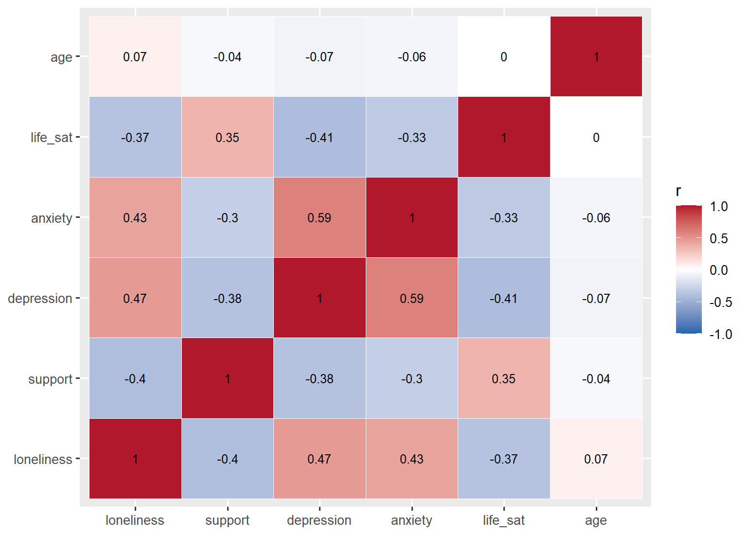
as.table() treats the matrix as a table and as.data.frame() turns it into a long data frame with one row per pair (36 rows), because geom_tile() draws one square per row, with var1 mapped to x, var2 to y and r to fill. scale_fill_gradient2() sets a diverging scale with white at zero, and limits = c(-1, 1) fixes its ends at the possible range of r.
set.seed(2021)
p_scatter <- ggplot(brief, aes(x = support, y = loneliness)) +
  geom_jitter(height = 0.2, width = 0, alpha = 0.15) +
  geom_smooth(method = "lm", colour = "#CC0033") +
  labs(x = "Social support (1 to 7)", y = "Loneliness score (3 to 9)")
ggMarginal(p_scatter, type = "histogram")    # a histogram on each axis
head(sort(table(brief$support), decreasing = TRUE), 3)   # the tallest spikes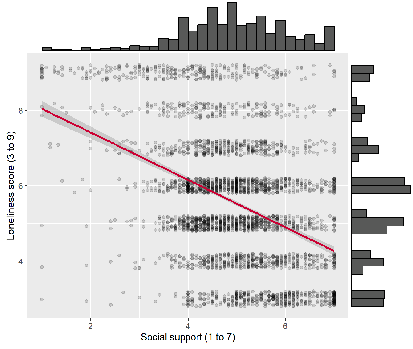
The message appears twice because ggMarginal() builds the scatterplot twice while it adds the margins; it is not an error. The histogram of support along the top is skewed to the left, with most people between 4 and 6 and a long, thin tail toward low support, and it has spikes at whole-number scores: 170 people score exactly 5, 136 exactly 4 and 117 exactly 7. A whole-number score is what a person who gives the same answer to all twelve support items receives. ggMarginal() returns a finished drawing, not a ggplot2 object, so patchwork cannot place it in a grid without extra steps, and the combined figure uses p_scatter without its margins.
p_hist <- ggplot(brief, aes(x = loneliness)) +
  geom_histogram(binwidth = 1, fill = "#0B7B6B", colour = "white") +
  labs(x = "Loneliness score (3 to 9)", y = "Number of people")
p_box <- ggplot(brief, aes(x = age_group, y = loneliness)) +
  geom_boxplot(fill = "#E6F3F0") +
  labs(x = "Age group", y = "Loneliness score (3 to 9)")
figure <- (p_hist + p_box) / (p_scatter + p_heat) +   # + side by side, / stacked
  plot_annotation(tag_levels = "A",                     # label the panels A to D
    title = "Loneliness and social connection, CSCS 2021 (n = 3,083)")
figure
ggsave("briefing_figure.png", figure, width = 11, height = 8.5, dpi = 300)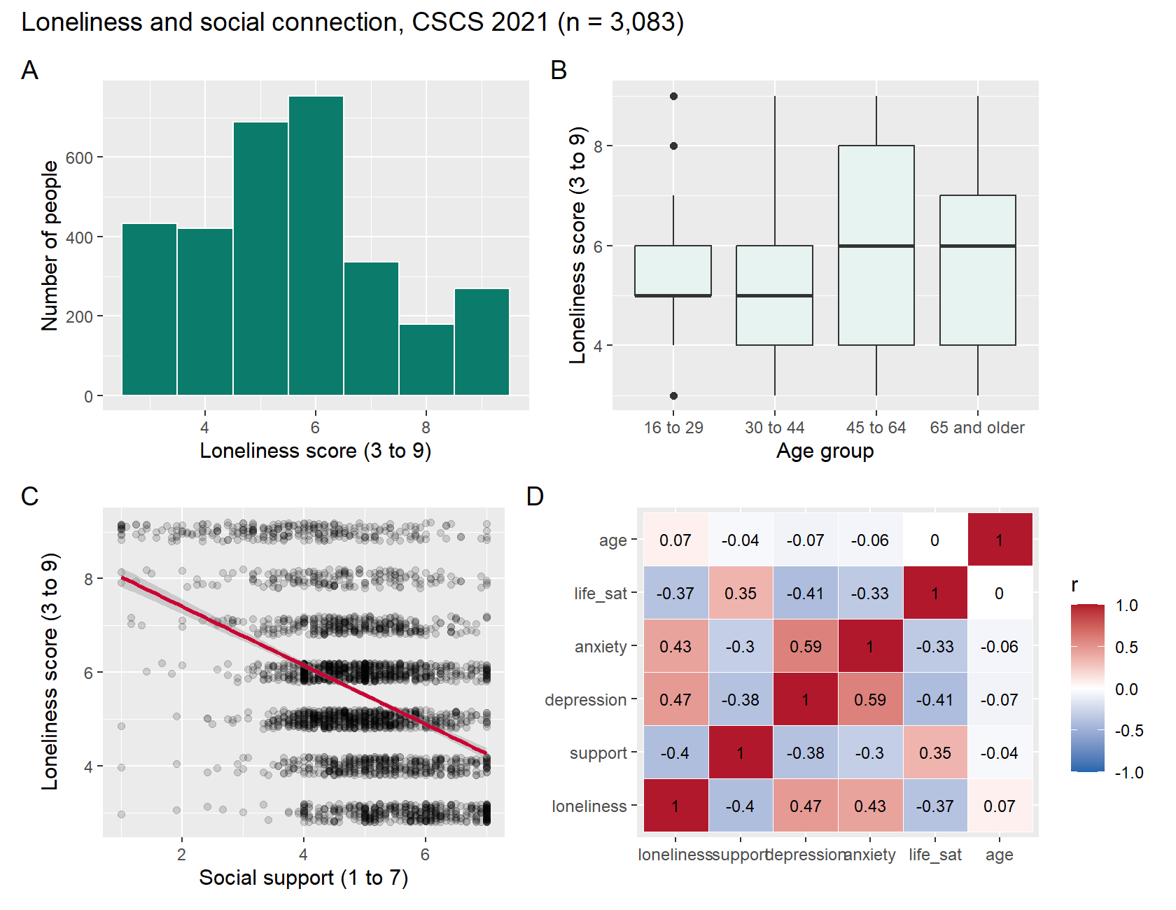
The plus sign places two plots side by side, the parentheses group each pair, and the forward slash stacks the two rows, giving a two-by-two grid. plot_annotation(tag_levels = "A") labels the panels A to D in reading order and adds the title. Typing figure draws the figure and ggsave() draws it again to save it, so the message from the scatterplot panel appears twice. The file is 11 by 8.5 inches at 300 dots per inch, or 3,300 by 2,550 pixels.
R Reflect on what you just ran
Answer each question from your own output, as on the final exam: read the matrix, say what a correlation can and cannot show, and check and caption the figure.
1. From cor_mat, which variable is most strongly related to loneliness, and in which direction? Interpret that correlation in one sentence. Social support is skewed: why is the Spearman correlation of loneliness with support (−0.36) useful here, and what does it show beside the Pearson value?
2. A member of the working group reads the heatmap and writes: “Social support reduces loneliness (r = −0.40), and age is unrelated to loneliness (r = 0.07).” Respond to both claims, and say what you would look at next.
3. Run your own code: at the end of your script, type figure & theme_minimal() and run it. What does & do, and which convention of a publication figure does the figure still not meet? Then write a caption for the figure that would let a reader understand it without reading the text.
& applies theme_minimal() to all four panels, giving them one plain theme (a plus sign would change only the last panel); panel D still shows R names such as life_sat, which should be replaced with plain labels such as “Life satisfaction”. Caption: Loneliness and social connection among respondents to the 2021 wave of the Canadian Social Connection Survey (n = 3,083 with complete data on all variables shown; 962 of 4,045 respondents were excluded for missing data). (A) Distribution of the three-item UCLA Loneliness Scale score (range 3 to 9; higher scores mean more loneliness). (B) Loneliness score by age group; boxes show the median and interquartile range, whiskers extend to the most extreme values within 1.5 times the interquartile range, and points show values beyond the whiskers. (C) Loneliness score against perceived social support (range 1 to 7); points are jittered vertically and drawn with transparency, and the line is a least-squares line with its 95% confidence band. (D) Pearson correlations among loneliness, social support, depressive symptoms (PHQ-2, 0 to 6), anxiety symptoms (GAD-2, 0 to 6), life satisfaction (1 to 10) and age, from blue (negative) through white (zero) to red (positive). The caption describes the figure and makes no causal claim; which differences matter belongs in the results text.Your output reproduces Table 6.7 and Figures 6.19 to 6.21, so each step of the section, from a single correlation to a captioned figure, has now been carried out on the briefing data.
This section has summarized many variables with a correlation matrix and a heatmap, set out the limits of that summary, added marginal histograms to a scatterplot, combined the briefing plots into one figure, and described the conventions of a publication figure and its caption. The key takeaways below summarize these ideas, the knowledge check reviews them, and the final page of the lesson brings the four sections together before the final assessment.
Key Takeaways
- 6.1 A correlation matrix, produced by
cor()on a set of numeric columns, gives Pearson's r for every pair of variables. Its diagonal is always 1, the values above the diagonal repeat those below it, and k variables give k(k − 1)/2 distinct correlations (15 for the six briefing variables). A heatmap draws each cell as a coloured square on a diverging scale (blue for negative, white at zero and red for positive, withlimits = c(-1, 1)), after the matrix has been reshaped into one row per pair and drawn withgeom_tile(). To interpret a correlation, give its direction from the sign and its strength from its size, using Cohen's rough guide of about 0.1, 0.3 and 0.5 for small, medium and large, and put it into words about people: r = −0.40 means that people with more social support tend to report less loneliness, a moderate negative association. When asked for the strongest correlation with a variable, read along its row, skip the 1 on the diagonal, and compare the sizes whatever their sign. - 6.2 Pearson's r measures straight-line association between numeric variables, and it can be pulled about by outliers and skew. Spearman's rank correlation, from
cor(..., method = "spearman"), works on the ranks of the values instead, so it is preferred for ordinal scores, skewed variables, and variables with extreme or piled-up values. Comparing the two is a useful check: for loneliness and social support, Spearman's value is −0.36 and Pearson's is −0.40, so the Pearson value is not being driven by a few extreme values. When the two differ noticeably, look at a scatterplot before reporting either number. In an exam question, the cue for Spearman is usually in the description of the variable: an ordered rating, a strongly skewed count, or a long tail of extreme values. - 6.3 A correlation heatmap shows the direction and strength of straight-line association between pairs of variables, and three common readings go beyond that. It cannot show a cause: the correlation of 0.47 between loneliness and depressive symptoms fits loneliness raising depressive symptoms, depression leading people to withdraw and feel lonelier (reverse causation), or a common cause such as poor physical health raising both (confounding), and a survey collected at one time cannot establish the order of events. A correlation near zero does not mean no relationship: age and loneliness have r = 0.07, yet the loess curve in Section 3 showed loneliness dipping around age 30, rising into the fifties and falling after 70, and these rises and falls cancel out in a single straight-line summary. And one number hides the shape of the data, including outliers, clusters, floors and ceilings and how many people contributed, as Anscombe's quartet showed. So when someone says a correlation shows that one variable reduces another, or that two variables are unrelated, reply that the correlation shows association only, name the other explanation (reverse causation, confounding or a curve), and ask for a scatterplot of that pair.
- 6.4 A scatterplot with marginal histograms shows a relationship and both distributions at once: the scatterplot sits in the middle, with a histogram of the horizontal variable along the top and a histogram of the vertical variable along the right side. In R, you build an ordinary ggplot2 scatterplot and pass it to
ggMarginal(p_scatter, type = "histogram")from the ggExtra package ("density"and"boxplot"are the other types). Read it in two steps: describe the relationship in the middle, then describe each margin for skew, spikes or piled-up values. In Figure 6.20, the margin showed that social support is skewed to the left and has spikes at whole-number scores (170 people at exactly 5), which is the score a person receives by giving the same answer to all twelve items, and a reason to look more closely before analyzing the score. Note thatggMarginal()returns a finished drawing, not a ggplot2 object, so you cannot add layers to it or place it in a patchwork grid without extra steps. - 7.1 The patchwork package combines finished ggplot2 plots into one figure with simple operators:
+or|places plots side by side,/stacks them, and parentheses group them, so(p_hist + p_box) / (p_scatter + p_heat)gives two plots on top and two below.plot_annotation(tag_levels = "A")labels the panels A, B, C and D in reading order so that the caption can refer to them, and the figure is saved withggsave()at a size that keeps every panel's text legible (11 by 8.5 inches at 300 dpi for the briefing). Before calling a figure finished, check it against the conventions in Table 6.8: axis labels in words with units or ranges, plain names rather than R names such aslife_sat, panel letters, legends that name their scale, colour-blind-safe colours, legible text, about 300 dpi, the sample size, and no chartjunk. When asked to critique a combined figure, work through that list, name each convention that is not met, and say how you would fix it. - 7.2 A caption is what lets a figure stand on its own, so that a reader can understand it without the text. It states what the figure shows and for whom: the data source and year, the number of people included and why others were excluded, the measures with their ranges, and what every panel and mark means (boxes, whiskers, points, lines and bands, and whether the points were jittered). It describes rather than interprets: which differences matter belongs in the results text, and a survey collected at one time cannot support a causal claim such as "loneliness causes depression". When you write or check a caption, test it against the four common failings (a causal claim; R names in place of plain measures; no source, year or number of people; and panels or marks that are not explained), and use the caption in Worked Example 6.1 as your model.
1. An analyst prints the Pearson correlations among five variables from a community health survey of 1,500 adults: daily steps, body mass index, systolic blood pressure, a stress score and age. Which statement correctly describes the strongest correlation with the stress score?
> round(cor(dat[, c("steps", "bmi", "sbp", "stress", "age")]), 2)
       steps   bmi   sbp stress   age
steps   1.00 -0.31 -0.18  -0.42 -0.25
bmi    -0.31  1.00  0.36   0.12  0.15
sbp    -0.18  0.36  1.00   0.09  0.48
stress -0.42  0.12  0.09   1.00 -0.05
age    -0.25  0.15  0.48  -0.05  1.00
2. A colleague reads a correlation heatmap from the same survey, which was collected at one time, and writes two sentences: "Age is unrelated to stress (r = −0.05). Walking more lowers stress (r = −0.42), so a walking program will reduce stress." Which response is correct?
3. A scatterplot of systolic blood pressure against the number of alcoholic drinks in the past week has marginal histograms added with ggMarginal(p, type = "histogram"). The histogram along the top shows drinks piled up near zero with a long right tail and about 15 adults above 40 drinks; the histogram on the right shows blood pressure as roughly symmetric. The Pearson correlation is 0.16 and the Spearman correlation is 0.06. Which interpretation is correct?
4. A colleague combined four plots with (p_a + p_b) / (p_c + p_d) + plot_annotation(tag_levels = "A") and saved the result with ggsave("draft.png", figure, width = 11, height = 8.5, dpi = 72). In the draft, the axes of panel D show the R names sbp and steps_day, and panel C colours women red and men green. Which assessment against the conventions of a publication figure is correct?
tag_levels = "A" labels the panels A to D in reading order, as the convention requires. The layout option misreads patchwork: + places two plots side by side, the parentheses group each pair, and / stacks the two rows, giving a two-by-two grid. (Section 4, 7.1.1 Combining Panels with patchwork and 7.1.2 Conventions of a Publication Figure, Table 6.8; Objective 7.1)5. A two-panel figure from a 2024 community health survey shows (A) a histogram of self-reported daily steps and (B) boxplots of systolic blood pressure for three age groups, with each adult drawn as a jittered point. Of the 1,900 adults surveyed, 1,640 had complete data. Which caption lets the figure stand on its own?
6. A survey of 1,120 staff in long-term care homes recorded weekly overtime hours, usual sleep (hours per night), a burnout score (0 to 30, higher means more burnout), days of sick leave in the past year (most staff took 0 to 3 days, and a few took more than 40) and age. Which summary of the output below is correct?
> round(cor(staff[, vars]), 2)
          overtime sleep burnout sick_days   age
overtime      1.00 -0.31    0.44      0.18 -0.12
sleep        -0.31  1.00   -0.52     -0.15  0.05
burnout       0.44 -0.52    1.00      0.26 -0.03
sick_days     0.18 -0.15    0.26      1.00  0.09
age          -0.12  0.05   -0.03      0.09  1.00
> round(cor(staff$burnout, staff$sick_days, method = "spearman"), 2)
[1] 0.14
Lesson 6: Final Assessment
Bringing It All Together
This lesson followed one request from start to finish: a one-page visual briefing on social connection for a regional loneliness working group, drawn from the 2021 wave of the Canadian Social Connection Survey. Section 1 set out why the analyst looks before modelling. Anscombe's quartet showed four datasets with the same means, standard deviations, correlation and fitted line but completely different patterns, and a decision guide matched the display to the number and types of the variables in a question. A gallery of poor displays showed what a truncated axis, a bar chart of means, a crowded pie chart and an overplotted scatterplot conceal.
Section 2 prepared the briefing file in base R (3,083 people with complete data on nine variables) and used quick base R plots to check it. A histogram revealed a spike of 116 people at the top value of household size, where larger totals had been recorded as 20, and heaping at 40 hours in reported hours of work, problems that the numeric summaries did not show. Section 3 rebuilt the plots with ggplot2, using the layered grammar of data, aesthetics, geoms, scales, facets and themes. A loess smoother showed that loneliness dips around age 30 and rises to a second high point in the fifties, facets compared the relationship between social support and loneliness across gender and age groups, and the Okabe-Ito palette kept the colours readable. Section 4 summarized many variables with a correlation heatmap, explained why a heatmap shows association and cannot show cause, curves or shape, added marginal histograms to a scatterplot, and combined four panels into one figure with a caption.
The same habits apply to every analysis: each variable is plotted before it is summarized, each relationship is plotted before it is modelled, and each figure carries labels and a caption that let it stand on its own. One question remains open: whether the scale scores plotted here, such as the loneliness and social support scores, measure what they are meant to measure, and how reliably they do so.
Key Takeaways from this lesson
- You can explain why exploratory analysis comes first: it uses plots and simple summaries to see the shape of each variable, any unusual values and the relationships between variables before a model is fitted, whereas confirmatory analysis tests a question set in advance. Anscombe's quartet shows why this matters, because four very different datasets share the same means, standard deviations, correlation and fitted line. Whenever an exam question gives you only summary numbers, say what a plot could reveal that the numbers cannot.
- You can choose a display by first naming how many variables a question involves and what type each one is: a histogram or a bar chart for one variable; a scatterplot, boxplots with points or a bar chart of percentages for two; and a correlation heatmap, a scatterplot matrix or facets for many. You can also decide between colour, for two or three groups that overlap little, and separate panels, for many, overlapping or unequal groups. The most useful reminder is to identify the variable types before naming the display, and to compare percentages within groups when the groups differ in size.
- You can spot a truncated bar axis, bars of means without spread, a pie chart with many slices, overplotting, a dual axis and colours that rely on telling red from green, explain what each one hides, and propose a better display. In a critique question, give each problem, what a reader could get wrong because of it, and its fix, and check the labels, the colours and the context (sample size and data source) as well as the type of display.
- You can read a histogram for skew, ceilings, heaping, top-coding, impossible values and missing-value codes, and a boxplot for centre, spread, skew and points beyond the whiskers. For every data problem you can respond by checking the codebook, deciding how to handle the problem, and reporting the decision with the number of people affected. Remember that points beyond the whiskers are flagged, not wrong, and that a right-skewed count with a variance well above its mean points toward a count model.
- You can read base R or ggplot2 code line by line and say in plain words what each part does for the figure: which variables are mapped to the axes, colour or fill; what the boxes, the jittered see-through points and the smoothed lines with their confidence bands show; and what facets, palettes, themes and saving with code add. You can then describe what the figure shows, including how many people sit behind each panel. The most useful reminder is that the grey band shows uncertainty about the average, not the spread of people, and that small panels are shown and their size stated, but they are not over-interpreted.
- You can read a correlation matrix, a correlation heatmap and a scatterplot with marginal histograms, describe a correlation by its direction and strength in plain words about people, and say when Spearman's rank correlation is preferred to Pearson's r. You can also explain why a correlation cannot show a cause, a curved relationship or the shape of the data. When someone draws a causal or "unrelated" conclusion from a correlation, name the other explanation and ask for a scatterplot of the pair.
- You can check a combined multi-panel figure against the conventions of a publication figure (plain labels with units, panel letters, named legends, colour-blind-safe colours, legible text, about 300 dpi, the sample size and no chartjunk) and write a caption that lets it stand on its own. The caption states the data source and year, the number of people and who was excluded, the measures and their ranges, and what every panel and mark means, and it describes rather than interprets, leaving any conclusion to the results text.
The final assessment covers all four sections. All 16 questions must be answered correctly (100%) to finish the lesson.
Final Knowledge Assessment
1. A colleague reports that the correlation between minutes of daily physical activity and resting heart rate is −0.80, gives the fitted straight line, and says that no plot is needed because "the numbers say it all". Which reply is best?
2. A briefing must compare the distribution of life satisfaction (whole numbers from 1 to 10) across four household income groups, which hold between 220 and 1,150 respondents. Which display suits this best?
3. A survey asks whether respondents are up to date with routine vaccinations. The analyst prints the counts and the percentages within each area below. A colleague's bar chart of counts shows a much taller "not up to date" bar for urban respondents. Which statement is correct?
> table(dat$area, dat$vaccines)                       # counts

        Not up to date Up to date
  Rural             45        105
  Urban            270       1080
> round(100 * prop.table(table(dat$area, dat$vaccines), margin = 1), 1)   # percentages within each area

        Not up to date Up to date
  Rural             30         70
  Urban             20         80
4. A draft figure plots, for each month, emergency department visits for asthma (red line, left axis from 0 to 400 visits) and the mean concentration of fine particulate matter (blue line, right axis from 10 to 30 micrograms per cubic metre). The two lines cross in June, and a colleague writes that pollution "overtakes" asthma visits in June. Which response is correct?
5. A clinic report shows the main reason for 2,300 walk-in visits as a pie chart with 12 slices, several of them thin, and the manager cannot tell whether skin problems or minor injuries are more common. Which redesign is best?
6. A histogram of household income (in $1,000s per year) falls smoothly toward higher incomes and then shows a tall bar of 64 households at 250, the largest value. The codebook says that incomes of $250,000 or more were recorded as 250. What is this, and how should it be handled?
7. In a survey of adults who smoke, reported cigarettes per day pile up at 10, 20 and 40, with few answers at 9, 11, 19 or 21. What does this suggest, and how should the analysis treat it?
8. Boxplots of the number of emergency department visits in the past year, for four income groups, show medians of 2, 1, 1 and 0 (from the lowest to the highest income), long upper whiskers, short lower whiskers and many separate points above the boxes. For all respondents, R prints the output below. What do the plot and these numbers suggest?
> mean(dat$ed_visits)
[1] 1.6
> var(dat$ed_visits)
[1] 6.4
> var(dat$ed_visits) / mean(dat$ed_visits)   # variance divided by the mean
[1] 4
9. A figure was drawn with the code below. The factor smoker has the levels "Does not smoke" and "Smokes". Which plain-words description of colour = sex, geom_smooth(method = "lm") and facet_wrap(~ smoker) is correct?
ggplot(dat, aes(x = age, y = sbp, colour = sex)) +
  geom_jitter(width = 0.3, alpha = 0.2) +
  geom_smooth(method = "lm") +
  facet_wrap(~ smoker) +
  labs(x = "Age (years)", y = "Systolic blood pressure (mmHg)", colour = "Sex") +
  theme_minimal()
aes() is mapped, so colour = sex gives each sex its own colour and adds a legend, and because the mapping is in ggplot() the smoother inherits it and draws one line per sex; method = "lm" makes each line straight (least squares), with the grey 95% confidence band drawn by default; and facet_wrap(~ smoker) repeats the plot in one panel per level of smoker, sharing both axes so the panels can be compared. The first option is tempting, but it confuses a mapped aesthetic with a fixed setting (a fixed colour is written outside aes()) and confuses "lm" with "loess". (Section 3, 5.4.3 Reading a Figure's Code in Plain Words, Table 6.5, and 5.8 Comparing Groups with Facets; Objective 5.4)10. A scatterplot shows about 3,000 respondents, with age recorded in whole years and systolic blood pressure recorded to the nearest 2 mmHg. Why does the code draw the points with geom_jitter(width = 0.3, alpha = 0.2) rather than geom_point()?
geom_jitter() adds a small random shift to where each point is drawn, and alpha sets the opacity from 0 (invisible) to 1 (solid), so overlapping points build up into darker areas that show where most people are. The option about correcting ages is tempting, but jitter moves only the drawn positions; it neither corrects nor changes the recorded values, and every respondent is still drawn. (Section 3, 5.5.2 A Numeric Variable Across Groups, and Section 2, 5.2 Jitter and Transparency for Overplotted Points; Objectives 5.2 and 5.5)11. In a scatterplot of systolic blood pressure against age, geom_smooth(method = "lm") draws a straight line with a grey band that is narrow in the middle of the age range and wider at both ends, where there are fewer respondents. What does the band show, and what would geom_smooth(method = "lm", se = FALSE) change?
se = FALSE removes the band but keeps the line. The information needed is what geom_smooth() estimates: the average of y at each value of x, here as a straight least-squares line, with a band that shows the uncertainty about where that average lies. The band is not the spread of individual people, most of whom lie outside it, and it widens toward the ends of the age range because fewer respondents are there. The argument se = FALSE keeps the line and drops the band; it changes neither the line nor the data. The option describing the band as the range of 95% of individuals is the most common misreading, since a band for the average is much narrower than the spread of individual values. (Section 3, 5.7 Reading a Scatterplot with a Smoother; Objective 5.7)12. A figure maps three groups to the default ggplot2 colours, which include a red and a green. Some readers of the report have red-green colour-vision deficiency, and others will print it in black and white. Which plan keeps the three groups distinguishable for all readers?
theme_bw() option is tempting, but a theme changes the background, borders and text, not the colours mapped to the data, so the groups would still be told apart only by red and green. (Section 3, 5.9.1 Palettes and Themes; Objective 5.9)13. In the briefing file (n = 3,083), the Pearson correlation between social support and loneliness is −0.40. Which sentence is the best interpretation?
14. In a survey collected at one time, hours spent outdoors each week are correlated with depressive symptoms (r = −0.35), and depressive symptoms are correlated with days of work missed (r = 0.30). A manager concludes: "Time outdoors prevents depression, which prevents missed work, so an outdoor activity program will cut missed work." Which response is correct?
15. A draft caption reads: "Figure 3. (A) Distribution of loneliness scores (UCLA three-item scale, range 3 to 9). (B) Loneliness score by age group; boxes show the median and interquartile range, whiskers extend to the most extreme values within 1.5 times the interquartile range, and points are jittered." Which addition would most improve it, so that the figure stands on its own?
16. A regional food security survey compares psychological distress (Kessler-6 score, 0 to 24, higher means more distress) across four household income groups. A colleague's draft panel is a bar chart of the mean distress score in each income group, with the four bars coloured red, green, orange and brown and the vertical axis titled K6_total. Which critique names the three problems and their fixes?
K6_total is an R variable name with no range, so the axis is labelled in words with its range. The theme_minimal() option is tempting, but a theme changes the background, grid lines and text, not the colours mapped to the data, and the resolution does not change what the panel shows. (Section 1, 3.1.1 Four Displays That Conceal the Data, Means without spread tab, and 3.1.2 Smaller Faults in Draft Figures, and Section 3, 5.9.1 Palettes and Themes; Objective 3.1)✦ Before submitting: pass every section knowledge check (100%).