Data Cleaning &
Descriptive Analyses
Exploratory Data Analysis For Epidemiology
Learning objectives for this lesson:
- Identify common types of data errors, including coding faults in a raw data file, the stage of the data pipeline where each enters, and how each should be corrected.
- Classify a described pattern of missing data as missing completely at random (MCAR), missing at random (MAR) or missing not at random (MNAR), justify the classification, and explain the consequence of a complete-case analysis under each.
- Apply systematic cleaning checks (range, consistency and outlier checks), decide whether to keep, transform or exclude each flagged value, and record the rule in a cleaning log.
- Choose a method for handling missing data (complete-case analysis, single imputation or multiple imputation) that suits the plausible mechanism and the amount missing.
- Choose, obtain in R and interpret measures of central tendency, spread and shape (skewness and excess kurtosis) for each variable type and distribution, and describe the shape of the distribution that a summary implies.
- Construct and interpret descriptive tables for epidemiologic research: frequency tables, cross-tabulations with an odds ratio, and a Table 1 stratified by exposure.
- Select visualisations that suit the variable type and the question, and assess whether a variable is close enough to normal for parametric methods.
This course was developed by Dr. Kiffer G. Card based on Dohoo, I. R., Martin, S. W., & Stryhn, H. (2012). Methods in Epidemiologic Research. VER Inc.
Glossary: Key Terms, People & Concepts
📚 Reference page, available throughout the lesson
This glossary collects the key concepts, people, and ideas you will meet in this lesson. Use it as a reference while you work through the material, or as a review before assessments. Type in the search box to filter entries.
Data Quality & Types of Errors
Overview
A structured workflow takes raw data from collection to analysis-ready files. This lesson concentrates on two phases of that workflow: cleaning the data (detecting errors, handling missing values and deciding what to do with outliers) and producing descriptive analyses (the numerical summaries, tables and plots that every analysis report opens with). This section lays the groundwork for both. It traces where errors enter the data pipeline, names the common types of error and the coding faults that can be spotted in a raw file, sets out the three mechanisms by which values go missing and what each means for an analysis, and describes the variable types recorded in a data dictionary. It closes by introducing the course dataset and its codebook and taking a first look at the raw file in R.
Learning Objectives
- 1.1 Trace where errors enter the collection → entry → storage → analysis pipeline.
- 1.2 Distinguish between common error types (transcription, coding, logical inconsistency, out-of-range and duplicate; random vs. systematic; structural vs. value-level), recognise coding faults in a raw extract, and state how each is corrected.
- 2.1 Classify missing-data mechanisms (MCAR, MAR, MNAR), justify the classification, and explain what each implies for a complete-case analysis.
- 5.1 Describe variable types in epidemiologic data and the operations each type supports.
1.1 Where Errors Enter the Data Pipeline
Before any statistical analysis can begin, data travel through a pipeline of four stages: collection, entry, storage and analysis. Errors can be introduced at every stage, and knowing where a problem arose is the first step toward finding and correcting it. At the collection stage, errors may arise from poorly worded survey items, interviewer bias, instrument malfunction or participant misunderstanding. During data entry, when values are copied from a form or device into a file, transcription mistakes and coding errors are common. Storage introduces risks of data corruption, version-control problems and format incompatibilities. Finally, at the analysis stage, incorrect variable coding, inappropriate transformations and software errors can compromise results.
Data quality has several dimensions. Wang and Strong (1996) asked data users what quality meant to them and found many dimensions beyond accuracy. Four of them matter at every cleaning step and appear in the walkthrough above: accuracy (the values are correct), completeness (the values are present), timeliness (the values are current enough for the question) and consistency (the values are recorded in the same format and agree with each other). A fifth, relevance, asks whether the data suit the research question at all. The principle that ties the pipeline and these dimensions together is worth committing to memory.
The Quality of an Analysis Cannot Exceed the Quality of Its Data
The quality of your analysis can never exceed the quality of your data. Careful attention to data quality at each stage of the pipeline is a prerequisite for valid epidemiologic inference.
The errors introduced at these stages take several recognisable forms, and naming them is the subject of the next subsection.
1.2 Types of Data Errors and How They Are Corrected
1.2.1 Screening, Diagnosing and Editing
Errors in epidemiologic datasets take many forms. Van den Broeck, Argeseanu Cunningham, Eeckels, & Herbst (2005) describe data cleaning as a three-stage process of screening, diagnosing and editing that should be planned into the study design rather than improvised after collection. Screening means looking systematically for values that seem odd, such as an age of 220 or an empty cell where an answer was expected. Diagnosing means deciding what each odd value is: an error, a true but unusual value, or a missing-data code. Editing means acting on the diagnosis by correcting the value from the source document, setting it to missing, or leaving it unchanged, and recording the decision. Planning these steps before data collection allows the study team to build some of the checks into the data-entry system itself.
Screening is easier when the analyst knows what to look for. Five types of error account for most of what turns up: transcription errors, coding errors, logical inconsistencies, out-of-range values and duplicate records. Click each card below to see how each type arises, an example of it, and the check that usually finds it.
Each card names an error by what it looks like in the file, and each points to a different check: double data entry for transcription errors, comparison with the codebook for coding errors, cross-field rules for logical inconsistencies, range checks for out-of-range values, and matching on key identifiers for duplicates.
1.2.2 Random, Systematic, Structural and Value-Level Errors
The five error types describe what an error looks like in the file. Two further distinctions describe how an error behaves, and both affect what the analyst can do about it.
Random versus systematic error. A random error is an error whose direction cannot be predicted. By this we mean that any one value is as likely to be recorded too high as too low: a reader misjudges a blood pressure gauge by a few mmHg, sometimes upward and sometimes downward. Because the errors scatter in both directions, they add noise to the data. This widens the spread of the values and makes estimates less precise, so that a repeated study would give more variable answers. When many values are averaged, the upward and downward errors tend to cancel out, so the mean is not pushed in one direction. Random error is not harmless, however. When it affects an exposure, it blurs the difference between people with high and low exposure, and as a result the estimated association between exposure and outcome is weakened toward no effect. For example, if some heavy drinkers are recorded as moderate drinkers and some moderate drinkers as heavy drinkers, the two groups look more alike than they really are, and any difference in their outcomes shrinks. In addition, random error matters whenever a measurement is compared with a cut-off. If high blood pressure is defined as a systolic reading of 140 mmHg or more, a true reading of 138 recorded as 142 moves a person above the cut-off, so individual people are misclassified and the proportion above the cut-off changes, even though the mean is largely unaffected.
A systematic error, by contrast, pushes values in the same direction every time, as with a miscalibrated scale that adds 2 kg to every weight. Systematic errors do not cancel out when values are averaged, so they produce bias, meaning an estimate that is consistently too high or too low. Collecting more data does not help, because every new value carries the same error. The two kinds of error are also found in different ways. Range checks catch some random errors, such as an impossible value, whereas a systematic error usually leaves values that look plausible and can be found only by comparison with an outside source, such as a recalibrated instrument.
Structural versus value-level error. A structural error affects the layout of the file: a variable stored as text when it should be a number, two variables merged into one column, a record that appears twice, or a missing-data code such as -9 mixed in with real values. A value-level error affects a single cell, such as one blood pressure entered as 1,200. The distinction matters for the order in which problems are fixed. Structural problems are usually fixed first, because value-level checks such as range checks give misleading answers when a column has the wrong type or contains codes. For example, if blood pressure is stored as text because one cell reads "not measured", R treats the whole column as text, so summary() reports no minimum or maximum and a range check cannot work as intended, and if a missing-data code of 999 sits among real readings, a range check flags every coded cell as an impossible value rather than as a missing one. Once the structure is correct, each remaining odd value can be judged on its own.
1.2.3 Coding Faults in a Raw File
Many structural problems are coding faults: they are built into a file by the way its values were recorded, and they can be spotted by reading a few raw rows beside the data dictionary. The table of coding faults below lists five that appear often in survey files. Read each row from left to right, because a complete answer about a fault always has two halves: what the problem is and why it matters, and the correction that best practice calls for.
Coding faults. Five common coding faults in a raw survey file, why each matters, and how each is corrected.
| Coding fault | Example | Why it matters | Correction |
|---|---|---|---|
| A missing-value code that could be a real value | Number of children recorded as 9 for "don't know" | A family with nine children cannot be told apart from a non-response, and the code is averaged as if it were a count. | Use a code that can never be a real response, such as −999, declare it in the data dictionary, and convert it to NA in the analysis script. |
| A compound code (two pieces of information in one variable) | smoke_alc = 23, where the first digit is smoking status and the second is drinking frequency | The variable cannot be summarised or checked directly, and a missing code such as 99 splits into two values of 9 that look like real but out-of-range answers. | Split it into two variables, one piece of information each, with its own valid range and missing code. |
| Text in a numeric field | Hours of exercise recorded as "none" or "unknown" | R reads the whole column as text (chr), so no mean or range check works, and as.numeric() turns every text entry into NA. | Record each entry as the number it means ("none" becomes 0) or as missing ("unknown" becomes NA), and keep the column numeric. |
| Inconsistent or ambiguous date formats | 03/04/2025, 4 Apr 25 and 2025-04-05 in one column | 03/04/2025 can mean 3 April or 4 March, and ages or durations calculated from mixed formats are wrong. | Store dates as a date variable in one unambiguous format, YYYY-MM-DD, and state the format in the data dictionary. |
| Inconsistent missing values | Some unanswered items left blank and others coded 99 | A blank may mean "not asked", "refused" or "lost", and some codes are missed when missing values are converted. | Use one documented convention for every variable, never a blank, and return incomplete forms to the source for completion where possible. |
Every correction is made in a script that reads the untouched raw file and writes a new version of it, never by editing the raw file by hand, so that each change can be checked and repeated. The next section carries out these steps in R. The errors described so far affect values that are present in the file; the next subsection turns to values that are absent.
2.1 Missing-Data Mechanisms
Missing data are ubiquitous in epidemiologic research, and the mechanism by which values become missing matters as much as how many are missing, because it decides whether an analysis of the people who remain gives valid answers. A missing-data mechanism is the process that decides which values end up missing. By this we mean the answer to the question "why is this value absent, and is the reason connected to anything about the person?" Rubin (1976) identified three mechanisms, which differ in what the missingness depends on. Data are missing completely at random (MCAR) when missingness is unrelated to anything about the people, observed or not; the people with missing values are then simply a random subset of the sample. Data are missing at random (MAR) when missingness depends only on variables that are recorded in the file. For example, younger people may skip a question more often than older people, but among people of the same age, whether the answer is missing has nothing to do with what the answer would have been. Data are missing not at random (MNAR) when missingness depends on the missing value itself, as when people with the most severe symptoms are the least likely to report them. The names are easy to confuse, because "missing at random" does not mean that the missingness is unrelated to everything; it means that the missingness is random once the recorded variables are taken into account. Click each card below to see an example of each mechanism and what it implies for a complete-case analysis, which analyses only the people with no missing values.
The cards show that the three mechanisms differ in what the missingness depends on, and that difference is what a classification has to justify.
Classifying a described pattern. Two questions settle most cases. First, is the missingness related to anything about the people, observed or not? If it arises from something unrelated to them, such as an equipment failure on days or in households assigned without regard to who the participants were, the pattern is MCAR, and a complete-case analysis remains unbiased but is less precise because the sample is smaller. Second, if the missingness is related to the people, is it fully explained by variables recorded in the file, such as age or survey format? If so, the pattern is MAR: a complete-case analysis can be biased, because the people who remain differ from those who are lost, and multiple imputation that uses the variables that predict missingness can give valid estimates. If instead the missingness depends on the missing value itself, for example people with the worst symptoms declining to report them, the pattern is MNAR: a complete-case analysis is biased in a direction that can usually be reasoned out (here, symptoms would be understated), imputation under the MAR assumption does not correct it, and sensitivity analyses are needed. A good justification is one sentence that names what the missingness depends on.
One caution applies to every classification, and it is a common source of exam errors.
The Mechanism Is an Assumption
The missing data mechanism is an assumption that cannot be verified from the observed data alone. You should always conduct sensitivity analyses to assess how your results might change under different assumptions about the missing data mechanism.
The next section returns to these mechanisms when it compares methods for handling missing data. Recognising a value as missing or erroneous first requires a record of what each variable should contain, which is the role of the data dictionary and of the variable types it records.
5.1 Variable Types and the Data Dictionary
5.1.1 Data Dictionaries and Codebooks
A data dictionary (or codebook) is a structured document that describes every variable in a dataset: its name, label, type, valid range, coding scheme, and source. Maintaining a comprehensive data dictionary is essential for:
- Ensuring consistency across data entry operators
- Facilitating communication among research team members
- Supporting reproducibility when analyses are revisited months or years later
- Identifying and resolving coding discrepancies
5.1.2 Variable Types in Epidemiologic Data
Among the entries in a data dictionary, the type of each variable matters most for analysis, because correctly classifying variables is fundamental to choosing appropriate cleaning strategies and analytic methods. Epidemiologic data contain four main types: continuous, categorical (nominal or ordinal), binary and count variables. Click each card below to see what each type is, with examples, and the cleaning checks that suit it.
The type decides which operations make sense. Means, standard deviations and differences suit continuous variables. For a categorical variable stored as numbers, the numbers are only labels: if blood type is coded 1 = A, 2 = B, 3 = AB and 4 = O, a mean blood type of 2.4 describes no real blood type, so a nominal variable is summarised by the count and percentage in each category, and an ordinal variable by the same counts kept in their natural order. A binary variable is summarised as the number and percentage with the characteristic, and a count variable by its mean and variance or its median.
5.1.3 The Course Dataset and Its Codebook
The R activities in this lesson use phaa_survey.csv, a simulated cross-sectional survey of 800 adults. Table 2.1 is a codebook excerpt for the variables this lesson works with most. A hard limit marks values that cannot be correct for this survey; values beyond it are treated as errors. A soft limit marks values that are possible but unusual; values between a soft and a hard limit are flagged for investigation, checked against the source where possible, and kept unless they are shown to be wrong. The limits are the rules applied in this lesson.
Table 2.1. Codebook excerpt for the variables of phaa_survey.csv used most in this lesson, with hard limits, soft limits and missing-data codes.
| Variable | Type and units | Valid values (hard limits) | Soft limits (flag and check) | Missing code |
|---|---|---|---|---|
id | Text identifier | P0001 to P0800, each appearing once | None | Never missing |
age | Continuous; whole years | 18 to 100 (only adults were eligible) | Above 90 | Blank cell |
systolic_bp | Continuous; mmHg, whole numbers | 80 to 220 | Below 90 or above 180 | Blank cell |
bmi | Continuous; kg/m², one decimal | 13 to 60 | Below 16 or above 50 | Blank cell |
smoker | Binary; text | "Yes" (current smoker) or "No" | None | Blank cell |
dep1 to dep7 | Ordinal questionnaire items | 1 (Never) to 5 (Always); a higher value means a more frequent depressive symptom | None | Blank cell |
income | Ordered categories; text | "<25k", "25-50k", "50-75k", "75-100k", ">100k" | None | Blank cell |
In this file a missing value is an empty cell, which R reads as NA (not available). Many real files instead store codes such as -9 (refused) or 999 (not asked); the codebook is where such codes are declared, and the next section shows how to convert them before any analysis. A full codebook would also record each variable's source, such as the questionnaire item or the measurement protocol; in this simulated file every variable comes from a single survey record per participant.
The codebook tells the analyst what each variable should contain; checking what the file actually contains is done in R, which needs a little preparation first.
5.1.4 Getting Ready to Run R and Reading R Code
The R boxes in this lesson read the course file directly from the course website, so no data file needs to be saved before they are run. The setup steps below are needed once, before the first R box: installing the add-on packages and running each activity's code from a script.
Setup Before the First R Box
Each R box in this lesson can be run in RStudio or any R console on a computer with an internet connection. No data file needs to be downloaded first: each activity reads the course data directly from the course website, for example with read.csv("https://heal-learn.ca/r-activities/data/phaa_survey.csv"), so R does not need to be pointed at a folder. Two preparations are needed once, before the first box.
- Install the add-on packages used in this lesson by running
install.packages(c("psych", "tableone"))once; the optional multiple-imputation panel in the next section also needsinstall.packages("mice"). A package is a bundle of extra functions; installing copies it to the computer, andlibrary(psych)loads it at the start of each new R session. - Download the Code file from each R box and open it in RStudio, or open a new R script (File > New File > R Script) and copy the code from the box into it. Each Code file reads the data it needs from the website, so each activity runs on its own; within an activity the lines are run in order, because later lines use objects created by earlier ones.
The Data link in each R box gives a copy of the file for anyone who wants to open it in a spreadsheet. A saved copy is read only from R's working directory, the folder R is currently pointed at: getwd() prints that folder, and in RStudio the menu Session > Set Working Directory > Choose Directory changes it.
A line of code runs when the cursor is on it and Ctrl+Enter (Cmd+Return on a Mac) is pressed, and the result appears in the Console pane. Selecting several lines and pressing the same keys runs them together, and the Source button runs the whole script from top to bottom. Running one line at a time allows each result to be compared with the annotated output on this page.
The code shown on this page is the starter code for every activity and can be copied directly. The answer-key script linked in each activity box contains the same code together with worked answers, and it becomes available after the responses to that box are saved.
For a longer demonstration, open the narrated R walkthrough below, which applies the cleaning and descriptive steps of this lesson to a real survey, the Canadian Social Connection Survey.
Narrated R walkthrough: Data Cleaning and Descriptive Statistics in R
This walkthrough applies the steps of this lesson to the Canadian Social Connection Survey, one line at a time. It keeps the rows and columns an analysis needs, explores each variable before changing it, recodes and checks every recode, and then describes the data with summary statistics, plots, stratified tables and a Table 1.
Open the Data Cleaning and Descriptive Statistics in R walkthroughR code is a sequence of instructions. Most lines either create an object (a named result stored in memory) or ask R to display something. Table 2.2 lists the symbols and terms that appear throughout the R code of this lesson; refer back to it whenever a line of code is unclear.
Table 2.2. Symbols and terms that appear in the R code of this lesson, each with an example and its meaning.
| Symbol or term | Example | What it means |
|---|---|---|
<- | x <- c(4, 7, 9) | The arrow stores the result on its right under the name on its left. The example creates an object called x that holds three numbers. |
c() | c("age", "bmi") | The function c() combines values into a vector, an ordered list of values of the same type. |
| Functions and arguments | mean(x, na.rm = TRUE) | A function is a named command followed by parentheses. The values inside the parentheses are its arguments, and name = value sets an option. |
$ | phaa$age | The dollar sign picks one column out of a data frame (R's name for a table of rows and columns). phaa$age is the age column of the data frame phaa. |
[ ] | phaa$age[3]phaa[1:5, c("id", "age")] | Square brackets select elements. For a single column, [3] picks the third value. For a data frame, the part before the comma picks rows and the part after the comma picks columns, so the second example shows the ID and age of the first five people. |
== < > <= >= != | phaa$age < 18 | Comparisons return TRUE or FALSE for each value. A double equals sign tests whether two values are equal, and != tests whether they differ. |
| and & | phaa$age < 18 | phaa$age > 100 | The vertical bar means "or" and the ampersand means "and". The example is TRUE for any age below 18 or above 100. |
! | !is.na(phaa$bmi) | The exclamation mark turns TRUE into FALSE and FALSE into TRUE, so the example is TRUE wherever BMI is present. |
NA | phaa$bmi[phaa$bmi > 60] <- NA | NA is R's code for a missing value. The example replaces every BMI above 60 with a missing value. |
na.rm = TRUE | mean(phaa$age, na.rm = TRUE) | Most summary functions return NA when any value is missing. The argument na.rm = TRUE (remove NAs) tells the function to leave missing values out. |
~ | boxplot(systolic_bp ~ smoker, data = phaa) | The tilde reads as "by" or "depending on". The example draws systolic blood pressure separately for each smoking group. |
# | # a note for readers | Everything after # on a line is a comment for human readers, and R ignores it. |
library() | library(psych) | The function loads an installed package so that its functions can be used in the current session. |
5.1.5 A First Look at the Raw File
Screening begins by reading the raw file and comparing what arrived with the codebook in Table 2.1, which brings together the ideas of this section: the variable types, the error types and coding faults, and the missing values. A few commands do most of this work: dim() reports the number of rows and columns, str() (structure) lists each variable with its type and first few values, summary() gives the minimum, quartiles, mean and maximum of numeric variables, table() counts the values of a categorical variable, and colSums(is.na()) counts the missing values in each column (is.na() marks each missing cell as TRUE and colSums() adds up the TRUEs in each column). Activity 2.1 practises this first screen of phaa_survey.csv one part at a time and asks what each part of the output shows and what to do with it; run each part along with the box and compare your output with the notes.
Text version of the activity: the code of the run-along script, its console output and notes on reading it.
# Blank cells and the text "NA" become missing values (NA)
phaa <- read.csv("https://heal-learn.ca/r-activities/data/phaa_survey.csv",   # course data, read from the website
                 stringsAsFactors = FALSE, na.strings = c("", "NA"))
dim(phaa) # rows (people) and columns (variables)The file has 800 rows, one per participant, and 27 columns, one per variable, which matches the codebook. A different count would suggest an incomplete download or a different version of the file.
str(phaa)                 # each variable's type and first few values
table(phaa$income, useNA = "ifany") # income bands, stored as textThe label chr means text (character), int means whole numbers and num means numbers that can have decimals. Every variable has the storage type the codebook leads one to expect; a numeric variable listed as chr would signal text, such as "unknown", hiding in the column. Storage is not the same as type: income is an ordinal variable stored as text, so table() lists its bands in alphabetical order, and the questionnaire items dep1 to dep7 are ordinal items stored as whole numbers.
summary(phaa[, c("age", "systolic_bp", "bmi", "dep1")])
phaa[phaa$age < 18 | phaa$age > 100, c("id", "age")]       # valid: 18 to 100
phaa[phaa$systolic_bp < 80 | phaa$systolic_bp > 220,       # valid: 80 to 220
     c("id", "systolic_bp", "diastolic_bp")]
phaa[phaa$bmi < 13 | phaa$bmi > 60, c("id", "bmi")] # valid: 13 to 60The middle of each distribution (quartiles and median) looks ordinary, but five values break the hard limits of Table 2.1: ages of -3 (P0033) and 220 (P0612), systolic blood pressures of 300 (P0017) and 60 (P0245, whose diastolic pressure of 63 is higher than its systolic pressure) and a BMI of 95 (P0078). The next section diagnoses them and sets them to missing.
table(phaa$smoker, useNA = "ifany")   # counts for a text variable
sum(duplicated(phaa$id))              # IDs that appear more than once
colSums(is.na(phaa)) # missing values in each columnSmoking status takes only the two codes in the codebook, "No" (664) and "Yes" (136), with no missing values, so no recoding is needed; variants such as "yes" or "Y" would appear as extra categories. No ID appears twice. Five variables have missing values: income (35), physical activity (28), social support (20), and the items dep4 (15) and anx2 (15). These counts are the starting point for the missing-data decisions in the next section.
R Reflect on what you just ran
Answer each question from your own output, as on the midterm exam: find the value in the output, say what it means, and say what to do about it.
1. Using the output of str() and table() and the codebook in Table 2.1, state the type of age, smoker, income and dep1, and how R stores each. For household income, type round(100 * prop.table(table(phaa$income)), 1) at the end of the script and run it to print the percentage in each band; then state the measure of central tendency and the measure of spread you would report, and justify the choice with evidence from the output.
int); smoker is binary and is stored as text (chr, "Yes" or "No"). Income is ordinal (five ordered bands) but is stored as text, so R does not know the order and table() lists the bands alphabetically, with >100k second. The item dep1 is also ordinal (1 Never to 5 Always) but is stored as whole numbers, so R would average it as if the steps between answers were equal. The storage type therefore shows how R will treat a column, not what its values mean, so the type comes from the data dictionary; a numeric variable listed as chr would signal text hiding in it. For income, report the count and percentage in each band, in order, among the people with income data: the counts come from line 14 and the percentages from your prop.table() line (under 25k: 94, 12.3%; 25-50k: 159, 20.8%; 50-75k: 207, 27.1%; 75-100k: 170, 22.2%; over 100k: 135, 17.6%), with the modal band, 50-75k, as the typical value. Income is recorded in ordered categories, so a mean and standard deviation have no meaning; the spread is shown by the percentage distribution, and the 35 missing values are reported.2. The output shows values in three variables that break the hard limits in Table 2.1. Identify each faulty value with its ID, name the type of error it most likely is, and state the stage of the data pipeline where it most likely entered. Then state how each should be corrected, according to best practice.
NA in the cleaning script, keeping the row and the person's other variables. Every correction is made in a script that reads the untouched raw file and is recorded in the cleaning log (the rule, the IDs and the number of values changed); the raw file is never edited by hand.3. Run your own code: at the end of the script, type tapply(phaa$age, is.na(phaa$income), median) and run it. Three possible explanations for the 35 missing incomes are described below. For each, classify the mechanism as missing completely at random, missing at random or missing not at random; justify the classification in one sentence; and state the consequence of analysing complete cases only. (i) For one batch of paper forms, the copier left blank the page that held the income question, and the forms were copied in random order. (ii) Income is missing more often among younger and less educated respondents, both recorded in the file, and shows no further relationship to income once age and education are accounted for. (iii) Respondents with the highest incomes chose not to answer the income question. Finally, what does your output show, and can it tell you which explanation is true?
tapply() line gives a median age of 45 among those who reported income (FALSE) and 43 among those who did not (TRUE), so the missingness is barely related to age. The output cannot show which explanation is true: a clear difference would be evidence against MCAR, but no comparison of observed values can rule out MNAR, because it depends on the values that are missing; the mechanism is an assumption, so state it and check conclusions with sensitivity analyses.The first screen in Activity 2.1 found each kind of problem described in this section: values that break the codebook's limits, columns whose storage type must match the codebook, and gaps whose mechanism has to be judged before they are handled. This section has traced where errors enter the data pipeline, classified types of error and missing-data mechanisms, and described the variable types recorded in a data dictionary. The key takeaways below summarise each of these points, the knowledge check that follows reviews them, and the next section sets out the cleaning workflow that addresses the problems found.
Key Takeaways
- 1.1 Data travel through four stages before you analyse them (collection, entry, storage and analysis), and errors can enter at every one. A poorly worded question, interviewer bias or a faulty instrument causes problems at collection; transcription slips and wrong codes happen at entry; corrupted files, version mix-ups and format incompatibilities arise in storage; and incorrect recodes, inappropriate transformations or software errors appear at the analysis stage. This is why data quality is checked throughout a project rather than with one final glance at the finished file: the quality of your analysis can never exceed the quality of your data. When an example describes a problem, name the stage where it most likely entered, because that tells you where the check belongs and where a correct value might be recovered, such as the original paper form for an entry error.
- 1.2 Errors can be named by what they look like in the file: transcription errors (transposed digits, a shifted decimal point), coding errors (a wrong or reversed code), logical inconsistencies (fields that contradict each other, such as a diagnosis dated before birth), out-of-range values and duplicate records. They can also be described by how they behave: random errors add noise and reduce precision, systematic errors push values the same way and cause bias, structural errors affect a whole column or the layout of the file, and value-level errors affect a single cell (fix structural problems first, because range checks mislead when a column holds text or codes). When you are given a few raw rows and a data dictionary, read each column against its entry and look for the common coding faults: a missing code that could be a real value (9 for "don't know" in a count of children), a compound code that stores two pieces of information in one variable, text such as "none" in a numeric field, mixed or ambiguous date formats (is 03/04/2025 3 April or 4 March?), and blanks mixed with missing codes. For each fault, state the correction as well as the problem: an impossible missing code such as −999 declared in the dictionary and converted to
NA, one variable for each piece of information, the number the text means ("none" becomes 0), dates stored as YYYY-MM-DD, and one documented missing-value convention. Make every correction in a script that reads the untouched raw file, never by editing the raw file by hand. - 2.1 Why values are missing matters as much as how many are missing, and Rubin's three mechanisms give you the words for it. Data are missing completely at random (MCAR) when the missingness has nothing to do with the people, observed or not, as when a freezer fails at random; missing at random (MAR) when it depends only on variables recorded in the file, such as younger people skipping the income question; and missing not at random (MNAR) when it depends on the missing value itself, as when people with the worst symptoms decline to report them. To classify a described pattern, ask two questions: is the missingness related to anything about the people, and if so, is it fully explained by variables in the file? Then answer in three parts: the label, a one-sentence justification that names what the missingness depends on, and the consequence for a complete-case analysis, which is unbiased but less precise under MCAR, possibly biased under MAR (where multiple imputation using the variables that predict missingness can give valid estimates), and biased under MNAR in a direction you can usually reason out (with the worst symptoms missing, symptoms would be understated). Because the mechanism cannot be confirmed from the observed data, state it as an assumption and check your conclusions with sensitivity analyses.
- 5.1 Variables come in different types depending on what their values represent: continuous (any value in a range, such as blood pressure or BMI), categorical, which may be nominal (no order, such as blood type) or ordinal (a meaningful order, such as disease severity or income bands), binary (exactly two categories) and count (non-negative whole numbers, such as hospital visits). You cannot always tell a variable's type from how its values are stored: ordinal questionnaire items such as
dep1todep7are stored as numbers, binary variables may be stored as 0 and 1, and a numeric variable may arrive as text, so check the data dictionary, which records each variable's type, valid values and missing codes. In R,str()shows how each column is stored (chrfor text,intfor whole numbers,numfor numbers with decimals); this tells you how R will treat the column, not what its values mean, and a numeric variable listed aschris a sign that text is hiding in it. Once you know the type, match the check to it: range and shape checks for continuous variables, frequency tables for unexpected categories or misspellings, exactly two valid values for binary variables, and no negative or implausibly large values for counts.
1. A research assistant types paper questionnaires into a spreadsheet. On one form the participant wrote a weight of 68 kg, but the spreadsheet shows 86 kg. At which stage of the data pipeline did this error enter, what type of error is it, and which check is most likely to catch it?
2. A community organisation sends the raw extract and data dictionary below. A colleague proposes four corrections. Which one follows best practice?
id   sleep_hrs  smk_alc  start_date   exercise_min
101  7          21       2025-02-03   30
102  9          99       03/02/2025   none
103  6.5        3        4 Feb 25     45

Data dictionary as supplied
  sleep_hrs     hours of sleep on a typical night; 9 = refused
  smk_alc       first digit = smoking (1 never, 2 former, 3 current)
                second digit = alcohol use (1 none, 2 monthly, 3 weekly)
                99 = missing
  start_date    date of first visit
  exercise_min  minutes of exercise on a typical day
as.numeric() would turn true zeros into missing values (b). smk_alc is a compound code that should be split into a smoking variable and an alcohol variable, each with its own missing code, because 99 would otherwise split into two values of 9 and the single digit 3 in row 103 cannot be decoded (c). Corrections are made in a script that reads the untouched raw file, with dates stored in one unambiguous format such as YYYY-MM-DD (03/02/2025 could mean 3 February or 2 March), never by hand (d). (Section 1, 1.2.3 Coding Faults in a Raw File, table of coding faults; Objective 1.2)3. In a cohort of 1,600 adults, the 12-month depression score is missing for 15% of participants. Missingness is higher among younger participants and among those who live more than 50 km from the clinic, both recorded at baseline, and among people of the same age and distance it is unrelated to their depression score. Which classification and consequence are correct?
4. A data dictionary codes region as 1 = North, 2 = South, 3 = East and 4 = West. A colleague's summary table reports "Region, mean (SD): 2.4 (1.1)". What is the problem, and what should be reported instead?
● Complete the knowledge check to continue.
Data Cleaning Strategies
Overview
The previous section named the kinds of errors that can enter a dataset and the mechanisms by which values go missing. This section sets out the cleaning workflow that deals with them. It begins with a systematic verification pass of range, type and consistency checks, moves on to outliers and the decision to keep, transform or exclude a flagged value, and then covers transformations, derived variables and the cleaning of text fields. It shows how every one of these decisions is documented so that the cleaned dataset can be rebuilt from the raw file, and it ends with the choice of a method for handling the missing values that remain.
Learning Objectives
- 3.1 Run range, type, and consistency checks as a first systematic verification pass, distinguishing hard limits (impossible values) from soft limits (unusual but possible values).
- 3.2 Identify outliers with the IQR and z-score rules and decide whether to keep, transform, or exclude them, with reasons recorded.
- 3.3 Apply transformations and derive new variables without losing the audit trail back to the raw data.
- 3.4 Document every cleaning decision, as a rule in a script and a cleaning log, so that another analyst could reproduce your final dataset.
- 4.1 Choose an appropriate missing-data strategy (complete-case, single imputation, multiple imputation) given the plausible mechanism and the amount missing.
3.1 Systematic Verification: Range, Type and Consistency Checks
Data cleaning should follow a systematic, documented process. The goal is not to “fix” data arbitrarily but to identify and resolve genuine errors while preserving the integrity of valid observations. A first verification pass therefore applies rules that were decided before anyone looked at the data, taken from the codebook, rather than fixing whatever happens to catch the analyst's eye. A type check comes first: it confirms that each column is stored as the codebook expects, for example that age is a number rather than text, because, as the previous section explained, value-level checks give misleading answers when a column has the wrong type. In R, str() shows the storage type of every column. Three further kinds of check follow. Expand each panel below to see how range checks, consistency checks and cross-validation work, and note in particular the difference between a hard limit and a soft limit in the first panel.
Range checks verify that values fall within predefined valid or plausible bounds. For example, gestational age should be between approximately 20 and 44 weeks; human body temperature typically ranges from 35°C to 42°C.
Define both hard limits (biologically impossible values that should be flagged as errors) and soft limits (unusual but possible values that should be reviewed).
The two kinds of limit lead to different actions. A value beyond a hard limit is an error: it is corrected from the source document if possible and otherwise set to missing. A value between a soft limit and a hard limit is flagged for investigation: the analyst lists it, checks it against the source where possible, and keeps it unless it is shown to be wrong. The codebook excerpt in the previous section (Table 2.1) gives both kinds of limit for the course data.
Consistency checks examine whether values across multiple fields are logically compatible. Examples include verifying that discharge dates occur after admission dates, that a participant’s age is consistent with their reported date of birth, and that skip patterns in questionnaires are respected.
These checks often require domain knowledge about the relationships between variables. By this we mean that the rule cannot be read from any single column; the analyst has to know how the variables should relate to each other. For example, a skip pattern means that people who answer "never smoked" are not asked how many cigarettes they smoke per day, so a record with both "never smoked" and a value of 20 cigarettes contradicts itself, even though each answer is valid on its own. Writing such rules therefore depends on knowing the questionnaire and the subject matter as well as the data.
Cross-validation involves comparing data from multiple sources to verify accuracy. For example, comparing self-reported medication use with pharmacy dispensing records, or verifying diagnoses against medical chart reviews.
When discrepancies arise, establishing a hierarchy of data source reliability is essential for deciding which value to retain. A hierarchy of reliability is a ranking of the sources from the most to the least trustworthy for a particular variable, agreed in advance. For example, a study might decide that a diagnosis confirmed in the medical chart outranks a diagnosis reported by the participant, because the chart was recorded by a clinician at the time. Because the ranking is set before the discrepancies are examined, the analyst does not choose, case by case, whichever value happens to suit the expected result.
The panels describe three different questions: whether one value is possible (a range check), whether the values in one record agree with each other (a consistency check), and whether the file agrees with another source (cross-validation). A range check examines one variable at a time, so it cannot find a record in which each value is valid on its own but the values contradict each other; only a consistency check does that.
The hard limits are applied in part 3 of Activity 2.2, at the end of this section. This is the editing stage of the screening, diagnosing and editing sequence: the values were screened in Activity 2.1, diagnosed as impossible because they break a hard limit, and are then replaced, with each change listed first. In the course file two ages (−3 and 220), two systolic pressures (300 and 60 mmHg) and one BMI (95) break a hard limit; each is set to NA and its row is kept, so the person's other 26 variables remain available, whereas deleting the row would discard valid data and could bias the results if errors are not random. Values in the soft-limit zones are left as they are. The raw file itself is never overwritten: range-check rules change as an analyst learns more about the data, and an untouched raw file lets the cleaning be replayed from a known starting state.
Range checks identify values that cannot be correct, and the values they set to missing join those already missing in the raw file, which 4.1 returns to. Values that are possible but lie far from the rest of the data are outliers, the subject of the next subsection.
3.2 Identifying Outliers and Deciding What to Do With Them
3.2.1 The IQR and z-Score Rules
Outliers are observations that lie far from the bulk of the data. They may represent genuine extreme values, data errors, or observations from a different population. The visual tools used to spot them, including box plots, stem-and-leaf displays, and the broader practice of looking at data before modelling, trace back to Tukey (1977). Two numerical rules are in common use. The IQR rule flags values below Q1 − 1.5 × IQR or above Q3 + 1.5 × IQR (Equation 2.1), and the z-score rule flags values more than three standard deviations from the mean (Equation 2.2). Open each tab below to see the formula for each rule with a worked example, and the third tab for the visual checks that complement both.
The interquartile range (IQR) method defines outliers as values falling below Q1 − 1.5×IQR or above Q3 + 1.5×IQR, where Q1 and Q3 are the 25th and 75th percentiles, respectively.
Equation 2.1 gives the two bounds as formulas.
This method is robust to extreme values because it is based on percentiles rather than the mean and standard deviation. A statistic is called robust when a few unusual values have little effect on it. By this we mean that the quartiles depend only on where the values at the 25th and 75th percentiles fall in the sorted list, not on how far the most extreme values lie beyond them. For example, if the largest reading in a sample changed from 184 to 1,840 mmHg, Q1 and Q3, and therefore the fences, would not change at all, so the rule used to judge the extreme value is not distorted by that same value. Values beyond 3×IQR from the quartiles are sometimes termed “extreme outliers.”
Worked Example 2.1 shows where the quartiles, IQR and fences that R reports come from, using eleven systolic blood pressure readings, and Table 2.3 sets out what each quantity is.
Worked Example 2.1: IQR Fences for Eleven Readings
Eleven systolic blood pressure readings (mmHg), sorted from lowest to highest, are 96, 102, 106, 110, 112, 115, 118, 121, 125, 131 and 184.
Table 2.3. How the median, quartiles, IQR and fences of the eleven systolic blood pressure readings are formed.
| Step | Calculation | Result |
|---|---|---|
| Median: the middle (6th) value | 96, 102, 106, 110, 112, 115, 118, 121, 125, 131, 184 | 115 |
| Q1: halfway between the 3rd and 4th values | (106 + 110) / 2 | 108 |
| Q3: halfway between the 8th and 9th values | (121 + 125) / 2 | 123 |
| IQR | 123 − 108 | 15 |
| Lower fence | 108 − 1.5 × 15 = 108 − 22.5 | 85.5 |
| Upper fence | 123 + 1.5 × 15 = 123 + 22.5 | 145.5 |
| Values outside the fences | 184 is above 145.5 | 184 is flagged |
The reading of 184 mmHg is flagged for investigation. It also lies beyond Q3 + 3 × IQR = 168, so some texts would call it an extreme outlier. A systolic pressure of 184 mmHg is high but physiologically possible, so the next step is to check the source record, and the value is kept if it is confirmed. In practice these numbers are read from R rather than worked out: for the same eleven values quantile() reports Q1 = 108 and Q3 = 123, IQR() reports 15 and boxplot.stats(x)$out lists 184 as the only value beyond the fences, as part 2 of Activity 2.2, at the end of this section, shows. Textbooks differ slightly in how they place Q1 and Q3 for some sample sizes, so the quartiles that R prints are the ones to report.
The z-score method standardizes each observation as z = (x − mean) / SD. Values with |z| > 3 are commonly flagged as potential outliers.
Equation 2.2 gives the z-score as a formula.
This approach assumes an approximately normal distribution and can be misleading for heavily skewed data because the mean and SD are themselves influenced by outliers (the masking effect). Masking is the situation in which an extreme value hides itself, or hides other unusual values, from the rule meant to detect it. This happens because the z-score is calculated from the mean and SD of all the values, including the extreme ones. An extreme value pulls the mean towards itself and, because its squared distance from the mean is large, it inflates the SD. As a result every z-score becomes smaller, since each distance is now divided by a larger SD, and values that would otherwise exceed 3 can fall below it. The cut-off of 3 also rests on the normal distribution, so in a strongly right-skewed variable many genuine values in the long tail can be flagged while unusual low values are missed.
Worked Example 2.2 shows what the z-scores of two systolic blood pressure readings mean.
Worked Example 2.2: A z-Score
The standard deviation (SD) measures the typical distance of values from their mean; the next section explains how it is calculated. Suppose systolic blood pressure in a population has a mean of 120 mmHg and an SD of 15 mmHg. A reading of 180 mmHg has z = (180 − 120) / 15 = 60 / 15 = 4, so it lies four SDs above the mean. The absolute value |z|, the size of z ignoring its sign, is 4, which is above the usual cut-off of 3, so the reading is flagged. A reading of 135 mmHg has z = (135 − 120) / 15 = 1, one SD above the mean, which is ordinary. In a bell-shaped (normal) distribution about 99.7% of values lie within three SDs of the mean, which is why |z| > 3 is the conventional flag. In R, scale() converts every value of a variable to its z-score in one step, so in practice the z-scores are read from R output and the task is to decide which readings to investigate.
Visual inspection using boxplots, histograms, and scatterplots is often the most informative first step in outlier detection.
- Boxplots display the median, IQR, and individual outliers beyond the whiskers
- Histograms reveal gaps in the distribution that may indicate erroneous values
- Scatterplots can reveal bivariate outliers that appear normal when each variable is examined individually
Visual methods should complement, not replace, quantitative rules. Always investigate outliers before deciding to exclude them.
The two worked examples show the main difference between the rules: the IQR rule rests on percentiles, which a few extreme values barely move, whereas the z-score rule rests on the mean and SD, which extreme values pull towards themselves.
3.2.2 Visual Checks
A boxplot draws the IQR rule directly. Figure 2.1 shows a boxplot of systolic blood pressure with the IQR fences marked and the points beyond them flagged.

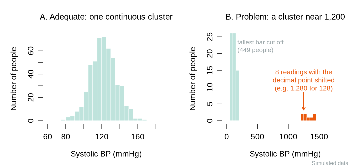
Two other kinds of problem are easier to see in a plot than in a table of numbers. A histogram (a bar chart of how many values fall in each range) shows gaps and separate clusters. When a decimal point is shifted during data entry, the shifted values form a small cluster at ten times the typical value, far from the main distribution, as in panel B of Figure 2.2.
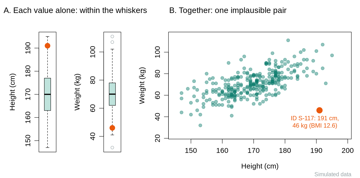
A scatter plot shows each person as a point with two measurements. A bivariate outlier is a combination of values that is implausible even though each value is ordinary on its own. In the simulated example in Figure 2.3, a height of 191 cm and a weight of 46 kg each lie inside the boxplot whiskers, but together they imply a BMI of 12.6, which would be life-threatening. Only the scatter plot reveals the problem.
3.2.3 Outlier Rules in R
Both numerical rules can be applied to a whole variable in a few lines of R. quantile(x, probs = c(0.25, 0.75)) returns Q1 and Q3, IQR() returns their difference, boxplot.stats(x)$out lists the values beyond the fences that a boxplot would draw as points, scale() converts every value to its z-score, and which() returns the row numbers where a condition is TRUE, so that the IDs can be listed. Part 2 of Activity 2.2, at the end of this section, repeats the eleven-reading example, applies the IQR rule and z-scores to BMI in the raw course file, and counts the values that fall in the soft-limit zones of the codebook. In the course file the IQR rule flags five BMI values, one impossible (95) and four ordinary values for adults with obesity (30.3 to 31.6), whereas the z rule flags only the 95: that single value pulls the mean up and inflates the SD from 3.24 to 4.17, and without it three of the four readings have |z| > 3. One extreme error hides other unusual values from the z rule, which is the masking described in the Z-Score tab. For skewed data, or whenever one value may be an error, the IQR rule is therefore the safer of the two.
3.2.4 Keep, Transform or Exclude
Every rule and plot in this subsection flags values; none of them can show that a value is wrong. The rule that follows is one of the most often tested in this lesson.
Never Delete an Outlier Because It Is Extreme
Never delete an outlier simply because it is extreme. Investigate whether it represents a data error, a genuinely unusual observation, or a member of a different subpopulation. Document every decision to retain or remove an outlier in your audit trail.
Once a flagged value has been investigated, one of three decisions follows. The panel below sets out when each applies and how the decision is written down as a rule in the cleaning log.
Keep, Transform or Exclude: Deciding What to Do With a Flagged Value
Keep a value that is possible and has been confirmed, or at least not shown to be wrong, such as a systolic pressure of 184 mmHg. If several such values give the variable a long tail, the variable is summarised with the median and IQR, or analysed with a rank-based method, rather than altered.
Transform the whole variable, not a single value, when its values are real but strongly skewed, for example ln(x + 1) for a right-skewed count that contains zeros (see 3.3 below). A transformation changes the scale of every value; it does not repair an error, so it is never the answer for an impossible or miscoded value.
Exclude a value that is an error: one beyond a hard limit, a missing-value code read as a number, or a value that the source document shows to be wrong. It is corrected from the source if possible and otherwise set to NA, and the row is kept so that the person's other values remain available. A whole row is removed only when the person falls outside the study population, and that criterion is stated in the methods.
Writing the rule. A cleaning-log rule names the variable, the limit or condition that was broken, the action taken, how many values it affected, and who made the change and when. For example: "systolic_bp outside the hard limits of 80 to 220 mmHg is impossible for this survey; values checked against the source records; 2 unverifiable values (300 and 60) set to NA; rows retained; AB, 2026-09-30." Activity 2.2, at the end of this section, records the same information as a table.
The outlier rules and soft limits flag values for investigation and leave them unchanged unless the investigation shows an error. Of the three decisions, transforming is the one that changes a whole variable, and it is the subject of the next subsection.
3.3 Transformations and Derived Variables
3.3.1 Transforming Skewed Variables
When continuous variables are heavily skewed, transformations can make the distribution more symmetric, stabilize variance, and improve the validity of parametric methods. A transformation applies the same mathematical function, such as the logarithm, to every value of a variable. By this we mean that, with the log and square-root transformations, the values keep their order but the distances between them change: on a log scale, for example, the step from 1 to 10 is the same size as the step from 10 to 100, so large values are pulled in much more than small ones. This is why a long right tail shrinks. Stabilizing variance refers to a related problem. In many skewed variables, such as biomarker concentrations, groups with higher averages also have much larger spreads, and a transformation that compresses large values can make the spreads of the groups more alike, which many methods assume. Parametric methods, such as the t-test and linear regression, assume that the data (or the errors of a model) follow a particular distribution, usually the bell-shaped normal distribution, which is fully described by its mean and standard deviation. When that assumption is badly wrong, their standard errors and confidence intervals can be misleading. Rank-based (non-parametric) methods, described in the next section, make fewer assumptions.
Figure 2.4 shows the effect of a natural-log transform on a right-skewed variable: the long right tail is pulled in and the distribution becomes roughly symmetric. Table 2.4 lists three common transformations with their formulas and typical uses.

Table 2.4. Three common transformations for skewed continuous variables, with their formulas and typical uses.
| Transformation | Formula | When to Use |
|---|---|---|
| Log (natural) | ln(x) or ln(x + 1) | Right-skewed data, multiplicative relationships (e.g., biomarker concentrations, income) |
| Square root | √x | Count data, moderately right-skewed distributions |
| Inverse (reciprocal) | 1/x | Strongly right-skewed data; commonly used for rates and times |
The log of zero does not exist (R returns -Inf, minus infinity), so a variable that contains zeros, such as the number of clinic visits, cannot be logged directly. The usual remedy is to add 1 to every value first, ln(x + 1), which turns 0 into ln(1) = 0 and keeps all values in the same order. The constant 1 is a convention; when most values are small, the choice of constant affects the results, and the report should state it. R has a dedicated function, log1p(), for ln(x + 1), and expm1() reverses it.
The reciprocal, 1/x, reverses the order of values: the largest value becomes the smallest. Analysts often use −1/x instead, so that larger original values still have larger transformed values and the direction of any association stays easy to read.
A transformed variable has to be interpreted on its new scale, and the results have to be returned to the original units before they are reported. The rule is general enough to commit to memory.
Interpret on the New Scale, Report on the Original Scale
When you transform a variable, all subsequent interpretations must account for the transformation. For example, a regression coefficient from a log-transformed outcome represents a multiplicative (rather than additive) change. By this we mean that the coefficient no longer says "the outcome is so many units higher"; it says "the outcome is so many times higher", or so many percent higher. This happens because equal steps on the log scale correspond to equal ratios on the original scale. Always back-transform results for reporting, so that readers see a value in the original units, such as mg/L, rather than a number on the log scale.
Worked Example 2.3 applies this rule to the simplest case, a mean calculated on the log scale; watch for which of the three numbers R prints is the one that goes in a report.
Worked Example 2.3: Back-Transforming a Log Mean
Nine C-reactive protein (CRP) values, a blood marker of inflammation, are 0.4, 0.8, 1.1, 1.5, 2.3, 3.0, 4.8, 9.5 and 21.0 mg/L. Part 5 of Activity 2.2 enters them in R. R prints an arithmetic mean of 4.93 mg/L, pulled upward by the single value of 21.0, and a median of 2.3 mg/L. On the log scale, mean(log(crp)) prints 0.906, and back-transforming with the exponential function, exp(mean(log(crp))), prints 2.48 mg/L. This back-transformed value is the geometric mean, a typical value on the original scale that is much less affected by the long right tail. A report would give the geometric mean of 2.48 mg/L, because the log-scale figure of 0.906 has no direct meaning for most readers. The same logic applies to regression coefficients for a log-transformed outcome, which are back-transformed into percentage differences.
The example shows that the geometric mean, unlike the arithmetic mean, stays close to the bulk of a right-skewed variable. Part 5 of Activity 2.2, at the end of this section, also demonstrates the other functions of this subsection: log() is the natural log and exp() reverses it, log1p() and expm1() are the matching pair for ln(x + 1), and the reciprocal reverses the order of 2, 5 and 10 (R prints 0.5, 0.2 and 0.1) while −1/x restores it.
3.3.2 Recoding and Derived Variables
A transformation changes the scale of an existing variable; recoding instead creates new variables from existing ones. Common examples include collapsing categories (e.g., combining “current smoker” and “former smoker” into “ever smoker”), categorizing continuous variables into clinically meaningful groups (e.g., BMI categories), and computing derived variables such as person-years of follow-up or age at onset.
In R, ifelse(condition, value_if_true, value_if_false) creates a new variable from a condition, and cut() turns a continuous variable into bands. In cut(), the breaks argument gives the cut-points, right = FALSE places each cut-point in the band above it (so a BMI of exactly 25.0 falls in the band 25 to 29.9), and labels names the bands. A cross-tabulation of the old and new variables, as in part 5 of Activity 2.2, is the standard check that a recode did what was intended. A derived variable is always stored as a new variable, so the original values are never overwritten and every result can be traced back to the raw data, and each new variable and its definition is added to the data dictionary.
3.3.3 String Cleaning and Duplicate Records
Free-text fields often contain inconsistencies: “Vancouver,” “vancouver,” “VANCOUVER,” and “Vancoouver” may all refer to the same city. Standardization strategies include converting to consistent case, trimming whitespace, applying regular expressions for pattern matching, and using lookup tables or fuzzy matching algorithms.
A regular expression is a short pattern that describes text. The pattern ^vanc means "text that starts with vanc" (the symbol ^ marks the start), and [0-9]+ means "one or more digits". The function grepl() asks whether a pattern occurs in each value, and gsub() replaces it. A lookup table is a two-column list that maps every known variant to its standard spelling. Fuzzy matching finds strings that differ by only a letter or two, which helps when the variants cannot all be listed in advance; its suggested matches should be checked by a person. The function duplicated() returns TRUE for the second and later copies of a value, so sum(duplicated(phaa$id)) counts repeated IDs.
Parts 5 and 6 of Activity 2.2, at the end of this section, apply these functions to five spellings of a city name, recode smoking status and BMI with ifelse() and cut(), and check the course file for repeated IDs. Lower case and trimws() merge three of the four spellings of Vancouver, and the pattern ^vanc catches the misspelling; a pattern this broad would also catch any other place name starting with "vanc", so the table is checked after every replacement. sum(duplicated(phaa$id)) is 0, so no ID appears twice; records entered twice under different IDs can be found with sum(duplicated(phaa[, names(phaa) != "id"])), which compares whole rows after setting the ID column aside and flags a record only when every other value matches. The recodes are stored in separate objects (city, smoker01, bmi_group) instead of new columns of phaa, so the cleaned file saved at the end of the lesson keeps the same columns as the course version of the dataset.
Every step so far, from range checks to recodes and text cleaning, changes or adds values, and each change has to be traceable. The next subsection sets out how these cleaning decisions are recorded.
3.4 Documenting the Cleaning Process
Every data cleaning decision should be recorded in an audit trail. This includes what was changed, why, by whom, and when. Reproducibility requires that another analyst could replicate the cleaning process from the original raw data using your documentation, an expectation echoed in the Statistical Methods in Psychology Journals guidelines (Wilkinson & the Task Force on Statistical Inference, 1999).
In practice the audit trail has two parts. The cleaning script records every change as code, with a comment giving the reason, and it is always run from the untouched raw file. A cleaning log, a small table with one row per changed value, records the date, the analyst, the ID, the variable, the old and new values and the reason, in a form that a reviewer can read without running any code. The cleaned data are then saved under a new file name so that the raw file is never overwritten; for the course data that file is phaa_survey_clean.csv, the survey after the range checks of this section, which Activity 2.3 in the next section reads from the course website.
An audit trail kept in a hypothetical cohort study of cardiovascular disease shows the two parts working together. The study collected blood pressure measurements on 2,400 participants, and during cleaning 15 systolic values exceeded 300 mmHg. The analyst traced 12 of these to a decimal-point shift (e.g., 1,200 instead of 120.0) and corrected them using the original paper forms. Three could not be verified and were set to missing with a note: “Original form illegible; value implausible.” All decisions were logged in a cleaning script with date stamps, so a reviewer could see every original value, every change and its reason, and could rebuild the cleaned file from the raw one. Correcting a value from the source document, as here, is good practice; what makes it acceptable is that the change is recorded and repeatable rather than typed over the raw file.
The range checks of 3.1 set five impossible values to missing, and they join the gaps that were already in the raw file. Deciding how to handle all of these missing values is the last step before the cleaned data are described, and it is the subject of the next subsection.
4.1 Choosing a Missing-Data Strategy
The choice of method for handling missing data depends on two things: the plausible missing-data mechanism, classified in the previous section as MCAR, MAR or MNAR, and the proportion of rows the analysis would lose. Practical guidance on implementing multiple imputation via chained equations, including how to specify the imputation model, how many imputations to draw, and how to diagnose problems, is given by White, Royston, & Wood (2011). The methods are compared in terms of five ideas, defined below, that recur whenever missing data are handled.
Five Terms for Comparing Missing-Data Methods
Complete-case analysis (also called listwise deletion) analyses only the rows that have no missing value on any variable used in the analysis.
Bias is a systematic difference between an estimate and the true value, so that repeating the study many times would give answers that are too high, or too low, on average.
Precision describes how much an estimate would vary from sample to sample; a precise estimate changes little when the study is repeated.
The standard error (SE) measures that sample-to-sample variation. For a mean it equals the standard deviation divided by the square root of the number of observations, so it shrinks as the sample grows.
A confidence interval (CI) is a range around an estimate, roughly the estimate plus or minus two standard errors for a 95% interval, that shows the values compatible with the data.
Missing data can damage both properties. Losing rows lowers precision (larger standard errors and wider confidence intervals), and missingness that is related to the values being studied, either directly (MNAR) or through observed variables linked to them (MAR), can bias a complete-case analysis.
Four methods are in common use, ranked here from the simplest to the one that handles uncertainty best: listwise deletion (complete-case analysis), pairwise deletion, single imputation and multiple imputation. Expand each panel below to see how each method works and where it goes wrong, paying particular attention to why single imputation makes standard errors too small and how multiple imputation avoids that.
Excludes any observation with one or more missing values. Simple to implement, but can dramatically reduce sample size and introduces bias unless data are MCAR. The bias arises because the people who remain are no longer a fair picture of the whole sample when missingness is related to who they are. For example, if younger people skip the income question more often, the complete cases contain too few young people, and any summary that depends on age is distorted. In multivariable models with many variables, even low rates of missingness on individual variables can lead to large cumulative losses. This happens because a person is dropped if any one of the variables is missing, and the gaps usually fall on different people, so the losses add up across variables. The course data show this in part 7 of Activity 2.2: no single column is missing more than 4.4% of its values, yet only 687 of the 800 rows are complete.
Uses all available data for each analysis. For example, when computing a correlation matrix, each pair of variables uses all cases with non-missing values for that pair. This preserves more data than listwise deletion, but can produce inconsistent results. For example, correlations computed on different subsets of people can form a set that could not all have come from one group of people (technically, a correlation matrix that is not positive semi-definite), which some later methods cannot use.
Mean imputation replaces missing values with the variable mean. While simple, it underestimates variance and distorts relationships between variables. The variance is underestimated because every filled-in value sits exactly at the centre of the distribution, so the data look less spread out than real values would be. For example, if 100 missing BMI values in a hypothetical study are all replaced by the same mean value, the variable gains 100 values with no distance from the mean at all. Relationships are distorted for a similar reason: the filled-in values ignore everything else known about each person, so a person with high blood pressure receives the same average BMI as a person with low blood pressure, and the association between the two variables is weakened. Median imputation is more robust for skewed distributions. Mode imputation is used for categorical variables.
All single imputation methods treat the imputed value as if it were known with certainty, leading to underestimated standard errors and overly narrow confidence intervals. By this we mean that the analysis cannot tell an imputed value from a measured one. It therefore counts the imputed values as real information, believes it has more data than it actually has, and reports its estimates as more precise than they really are.
Multiple imputation creates several (typically 5–20) plausible imputed datasets, analyzes each separately, and pools the results using Rubin’s rules. Each missing value is filled with a plausible value predicted from the person's other recorded variables, plus a random amount that reflects how uncertain that prediction is. Because the random part differs each time, the completed datasets differ slightly from one another in the values they fill in, while the observed values stay the same in all of them. This approach correctly accounts for the uncertainty due to missing data and produces valid inference under the MAR assumption.
Rubin’s rules average the estimates from the completed datasets and combine two sources of variation in the standard error: the ordinary variation within each dataset and the variation between datasets, which reflects how uncertain the imputed values are. By this we mean that if the completed datasets give very similar estimates, the missing values matter little and the pooled standard error is only slightly larger than it would be with complete data. If instead the estimates differ a lot from one dataset to the next, the missing values could plausibly have been quite different, and the pooled standard error grows to reflect that. This is the step that single imputation leaves out, and it is why multiple imputation does not overstate precision.
Multiple imputation is widely used for handling missing data in epidemiologic research when the proportion of missingness is non-trivial. It needs care: the imputation model should include the outcome and the variables that predict missingness (Sterne et al., 2009).
The panels set out the trade-off that drives the choice: the simpler methods either discard people or pretend to know values that were never recorded, while multiple imputation keeps everyone and carries the uncertainty about the missing values into the standard errors. Before any of them is applied, the analyst has to make sure that R recognises every missing value, then find out how much is missing and who is missing.
4.1.1 Missing-Data Codes Such as -9 and 999
Many data systems cannot leave a cell empty, so they store a code such as -9 (refused) or 999 (not asked) instead. R treats these codes as real numbers. A single age of 999 among the 800 ages in the course file would raise the mean by about 1.2 years, and in a small sample one code can move a mean by decades: in part 7 of Activity 2.2, at the end of this section, the mean of five ages that include the codes -9 and 999 is 224.4, while the mean of the three real ages is 44. The codebook lists the codes for each variable, and the analyst converts them to NA before any summary is calculated, for example with age_raw[age_raw %in% c(-9, 999)] <- NA. The course file uses empty cells only, so the activity uses a short made-up vector. The operator %in% asks, for each value on its left, whether it appears in the list on its right. The na.strings argument of read.csv(), for example na.strings = c("", "NA", "-9", "999"), converts codes while the file is read, but it applies to every column, so it is safe only when the code cannot be a real value in any column. A value of 999 could be a real number of minutes of activity per week, for example. Converting codes column by column with %in%, guided by the codebook, avoids that problem.
4.1.2 How Much Is Missing, and Who Is Missing?
Once every missing value is coded as NA, choosing a method starts with knowing how much is missing and whether the people with missing values differ from the rest. In R, colSums(is.na(phaa)) counts the missing values in each column, complete.cases() returns TRUE for each row with no missing value, na.omit() returns a copy of the data with every incomplete row removed, and tapply(y, group, mean) calculates the mean of y separately for each value of group. Part 7 of Activity 2.2, at the end of this section, uses these functions on the course file after the range checks. Eight columns then have gaps, the largest being income at 4.4%, yet only 687 of the 800 rows (85.9%) are complete: a complete-case analysis that used every column would lose 113 people (14%), because the gaps fall on different people, so na.omit() should be applied only to the columns an analysis needs, for example na.omit(phaa[, c("age", "systolic_bp")]). The 35 people without an income value are a little younger (42.6 versus 45.3 years), have slightly lower systolic BP (105.3 versus 108.4 mmHg) and smoke less often (8.6% versus 17.4%, which is 3 of the 35 people). Differences like these, if real, would argue against MCAR and suggest that missingness depends on observed variables (MAR). Because the course file is simulated, its true mechanism is known: the income values were deleted completely at random, so the differences arose by chance in a group of only 35 people. Comparisons of this kind can suggest a mechanism, and small groups can produce sizeable differences by chance alone, so they cannot establish one.
4.1.3 Reasoning About the Mechanism
The observed data can show that missingness is related to observed variables, which is evidence against MCAR. They cannot show whether missingness depends on the missing values themselves, because those values were never recorded. Whether MNAR is plausible is therefore judged from subject knowledge. Income is the standard example: refusal to answer income questions is often reported to be more common among people with high incomes, so an analyst should treat MNAR as a real possibility for income even when a comparison like the one in Activity 2.2 looks reassuring. By contrast, a blood pressure reading lost because a machine failed at random times is a case where MCAR is plausible.
Because the mechanism cannot be confirmed from the data, it is stated as an assumption in the methods section of a report. An example sentence is: "Income was missing for 35 of 800 participants (4.4%). We assumed that income was missing at random given age, gender, education and region, and handled it with multiple imputation; a sensitivity analysis that assumed non-responders had higher incomes than similar responders gave similar results." The sentence reports the amount missing, the assumed mechanism, the method used, and how the conclusion was checked.
A formal test of the MCAR assumption exists, but what it can show is limited, and over-reading it is a common mistake.
What Little’s MCAR Test Can and Cannot Show
Little’s test (Little, 1988) compares the means of the observed variables across groups of people with different patterns of missing values. A small p-value (a result that would be unlikely if the data were MCAR) is evidence that the data are not MCAR. A large p-value is weak reassurance: the test has little power (ability to detect a departure from MCAR) when few values are missing, and because it uses only observed values it cannot detect MNAR at all. The test is available in add-on R packages (for example as mcar_test() in the naniar package) and is not needed in this course; the group comparison in part 7 of Activity 2.2 examines the same question in a form that is easier to read.
Why the mechanism matters so much becomes clear when the same number of values goes missing in two different ways. Worked Example 2.4 compares a complete-case mean when the missing people are chosen at random with the same mean when the highest earners are the ones who do not answer; watch the direction of the error in each case.
Worked Example 2.4: Missing High Earners Bias the Mean
Ten people have annual incomes (in thousands of dollars) of 22, 28, 31, 35, 40, 46, 52, 60, 85 and 120, with a true mean of 51.9. Table 2.5 shows the complete-case mean of the eight people who remain when two of them do not answer.
Table 2.5. Complete-case means of the ten incomes when two people chosen at random, or the two highest earners, do not answer.
| Scenario | People who do not answer | Complete-case mean of the other eight | Error |
|---|---|---|---|
| Two people chosen at random (MCAR) | 31 and 52 | 54.5 | +2.6 |
| The two highest earners (MNAR) | 85 and 120 | 39.25 | −12.65 |
When the missing people are chosen at random (MCAR), the error can go in either direction and averages out to zero over many repetitions; the only cost is a smaller sample. When the highest values are the ones that go missing (MNAR), every complete-case mean is pulled downward, and collecting more data of the same kind does not remove the error. Part 8 of Activity 2.2, at the end of this section, repeats the comparison with 10,000 simulated incomes. There set.seed() fixes the random numbers so that the results repeat exactly, rlnorm() draws right-skewed values, and runif(10000) < 0.30 is TRUE for a random 30% of people. R prints a true mean of 65.9 thousand dollars. With MCAR missingness the complete-case mean that R prints, 65.3, is close to the truth, and the standard error rises from 0.437 to 0.509 because fewer values remain: no bias, lower precision. With MNAR missingness, where the top quarter of earners leave the question blank far more often, the line mean(inc_mnar, na.rm = TRUE) prints 54.4, well below the true mean of 65.9, and no method that uses only the observed incomes can recover the missing information without further assumptions.
The worked example shows that the amount missing was the same in both scenarios; only the mechanism differed, and it alone decided whether the complete-case mean was biased. The amount missing still matters for the choice of method, as the next part explains.
4.1.4 How Much Missing Data Is Too Much?
No single threshold applies to every study. As a rough guide, many applied texts suggest that when fewer than about 5% of the rows needed for an analysis have missing values and MCAR is plausible, complete-case analysis is unlikely to change the conclusions much. When more is missing, when missingness is related to observed variables, or when MNAR is plausible, multiple imputation under a stated MAR assumption, together with a sensitivity analysis, is the safer choice. The proportion that matters is the share of rows lost from the specific analysis, which can be much larger than the share missing on any one variable, as the 687 complete rows in part 7 of Activity 2.2 show.
This guide also explains where complete-case analysis fits in this lesson. It is defensible when little is missing and MCAR is plausible, which is the situation in the scale activity in the next section, where na.omit() drops the 15 people (about 2%) who skipped one depression item before a factor analysis. It becomes hard to defend when many rows are lost or when the people with missing values differ from the rest.
When the guide points to multiple imputation, the work is done in R. The optional panel below goes further than the course requires: expand it to see a minimal multiple imputation with the mice package, with its output read line by line and compared with a complete-case estimate.
The mice package (multivariate imputation by chained equations) fills each missing value with a draw from a model built from the other variables, repeats this to create several completed datasets, analyses each dataset, and pools the results with Rubin’s rules. The reference code below imputes the 28 missing physical-activity values using age, gender, smoking status, BMI and social support, and estimates the mean weekly activity. It runs after the code of Activity 2.2, so phaa holds the cleaned data, and it needs the mice package (install.packages("mice"), once).
library(mice)
mi_vars <- phaa[, c("age", "gender", "smoker", "bmi", "phys_act_min",
                    "social_support_score")]
mi_vars$gender <- factor(mi_vars$gender)
mi_vars$smoker <- factor(mi_vars$smoker)
imp <- mice(mi_vars, m = 5, seed = 2026, printFlag = FALSE)  # 5 completed datasets
fit <- with(imp, lm(phys_act_min ~ 1))   # lm(y ~ 1) estimates the mean of y
summary(pool(fit), conf.int = TRUE)      # pooled with Rubin's rules

# Complete-case estimate and its standard error, for comparison
mean(phaa$phys_act_min, na.rm = TRUE)
sd(phaa$phys_act_min, na.rm = TRUE) / sqrt(sum(!is.na(phaa$phys_act_min)))| Code or output | What it means |
|---|---|
mice(mi_vars, m = 5, seed = 2026, printFlag = FALSE) | The function creates five completed datasets; seed makes the random draws repeatable and printFlag = FALSE hides the progress messages. When the package loads, R prints messages about functions it masks, which can be ignored. |
with(imp, lm(phys_act_min ~ 1)) | The same analysis is run on each completed dataset. lm(y ~ 1) is a regression with no predictors, whose single coefficient (the intercept) is the mean of y. |
estimate, std.error, 2.5 % and 97.5 % | The pooled mean is 175.7 minutes per week with a standard error of 2.94 and a 95% confidence interval from 170.0 to 181.5. These are the numbers to report. |
| Complete-case mean and standard error | The complete-case mean is 176.1 (SE 2.96). The two answers agree closely, as expected, because the values in this simulated file were removed completely at random. With MAR missingness in real data the two can differ noticeably, and the imputed estimate is the one that corrects the bias when the MAR assumption holds. |
For a fuller demonstration on real survey data, open the narrated R walkthrough below, which applies the steps of this subsection, from counting and comparing missing values to multiple imputation, to the Canadian Social Connection Survey.
Narrated R walkthrough: Missing Data and Multiple Imputation in R
The walkthrough counts the missing values in a survey dataset and lists their patterns, compares people with and without gaps to judge which mechanism is plausible, compares the people who have an outcome with the people who do not, fits a complete-case model, shows what mean and mode imputation do to the data, and then creates 40 imputed datasets with mice() and pools the results with Rubin’s rules.
Every step of the cleaning workflow, from the first type check to the choice of a missing-data method, is now in place, and Activity 2.2 puts them together as one cleaning script. A cleaning script starts with a header that names the script, the raw file (which is never edited) and the file the script writes. Activity 2.2 practises the whole of this section in R on the raw course file: it checks the variable types, applies the outlier rules and the soft limits, replaces the values that break a hard limit, writes a cleaning log with one row for each value changed, transforms and recodes into new variables, cleans text, checks for duplicate IDs, and examines how much is missing and who is missing. Run the script along with the box, one part at a time, and compare each result with the notes.
Text version of the activity: the code of the run-along script, its console output and notes on reading it.
phaa <- read.csv("https://heal-learn.ca/r-activities/data/phaa_survey.csv",   # course data, read from the website
                 stringsAsFactors = FALSE, na.strings = c("", "NA"))
summary(phaa$age)                  # before the conversion
phaa$age <- as.numeric(phaa$age)   # text such as "unknown" would become NA
phaa$bmi <- as.numeric(phaa$bmi)
summary(phaa$age) # after the conversionThe file is the raw course file phaa_survey.csv, the simulated survey of 800 adults introduced in Section 1, read straight from the course website; the raw file is never edited, so the cleaning can always be replayed from a known starting state. na.strings = c("", "NA") treats blank cells as missing. In this file every age cell holds a number, so read.csv() already stores age as a number and both summaries show 0 NAs: the conversion changes nothing here. Had a cell held text such as "unknown" or "30s", the column would have arrived as character and as.numeric() would have turned each such cell into NA, with a warning. The minimum of −3 and the maximum of 220 are the first sign of impossible ages.
x <- c(96, 102, 106, 110, 112, 115, 118, 121, 125, 131, 184)
quantile(x, probs = c(0.25, 0.75))   # Q1 and Q3
IQR(x)                               # Q3 minus Q1
boxplot.stats(x)$out                 # values beyond the fences
q <- quantile(phaa$bmi, probs = c(0.25, 0.75), na.rm = TRUE)
fences <- c(q[1] - 1.5 * IQR(phaa$bmi), q[2] + 1.5 * IQR(phaa$bmi))
fences
phaa[which(phaa$bmi < fences[1] | phaa$bmi > fences[2]), c("id", "bmi")]
z <- as.numeric(scale(phaa$bmi))     # z = (x - mean) / SD
phaa$id[which(abs(z) > 3)]           # IDs with |z| above 3
round(z[which(phaa$bmi == 31.6)], 2)
bmi_ok <- phaa$bmi[phaa$bmi < 60]    # without the impossible 95
round(c(sd_all = sd(phaa$bmi), sd_ok = sd(bmi_ok)), 2)
round((c(30.6, 30.8, 31.6) - mean(bmi_ok)) / sd(bmi_ok), 2)
sum(phaa$systolic_bp < 90 | phaa$systolic_bp > 180)   # soft limits
sum(phaa$bmi < 16 | phaa$bmi > 50)For the eleven readings of Worked Example 2.1, R prints Q1 = 108, Q3 = 123 and IQR = 15, and only 184 lies beyond the fences. For BMI the fences are 11.45 and 30.25, and five values are flagged. One (95.0, ID P0078) is impossible; the other four (30.3 to 31.6) are ordinary values for adults with obesity. The IQR rule finds what is unusual in this sample, and it cannot tell an error from a real value. Only P0078 has |z| > 3: the single value of 95 pulls the mean up and inflates the SD from 3.24 to 4.17, so the BMI of 31.6 has z = 2.58. Without the impossible value, the readings of 30.6, 30.8 and 31.6 have z = 3.03, 3.09 and 3.34. One extreme error hid three unusual values from the z rule, which is called masking, and it is why the IQR rule is safer for skewed data. The soft-limit counts flag values for a second look and change nothing: 48 systolic readings lie below 90 or above 180 mmHg (two of them, 60 and 300, are beyond the hard limits; the other 46 lie between 85 and 89 mmHg), and 67 BMI values lie below 16 or above 50 (one is the impossible 95; the other 66 lie between 15.0 and 15.9 and are kept).
phaa[which(phaa$age < 18 | phaa$age > 100), c("id", "age")]
phaa[which(phaa$systolic_bp < 80 | phaa$systolic_bp > 220), c("id", "systolic_bp")]
phaa[which(phaa$bmi < 13 | phaa$bmi > 60), c("id", "bmi")]
phaa$age[phaa$age < 18 | phaa$age > 100] <- NA
phaa$systolic_bp[phaa$systolic_bp < 80 | phaa$systolic_bp > 220] <- NA
phaa$bmi[phaa$bmi < 13 | phaa$bmi > 60] <- NA
summary(phaa$age)                  # 2 NAs, and every row is kept
phaa$education <- factor(phaa$education, levels = c("Less than high school",
  "High school", "Some college", "Bachelor's", "Graduate degree"), ordered = TRUE)
levels(phaa$education) # lowest to highestThis is the editing stage of the screening, diagnosing and editing sequence. The first three lines list the values that break each hard limit in the codebook, with their IDs, before anything is changed: two ages (−3 and 220), two systolic pressures (300 and 60 mmHg) and one BMI (95). The next three lines replace them with NA. Replacing an impossible value with NA keeps the row, so the person's other 26 variables remain available, and the gap is then handled like any other missing value; deleting the row would discard valid data and could bias the results if errors are not random. summary(phaa$age) now shows 2 NAs while all 800 rows remain. Values in the soft-limit zones are left as they are. The last two lines make education an ordered factor, so that R treats "Less than high school" < "High school" < "Some college" < "Bachelor's" < "Graduate degree" as a direction; without the levels, R would sort the categories alphabetically, which makes no sense for a question such as "as education goes up, does blood pressure change?".
cleaning_log <- data.frame(date = "2026-09-30", analyst = "AB",
  id       = c("P0033", "P0612", "P0017", "P0245", "P0078"),
  variable = c("age", "age", "systolic_bp", "systolic_bp", "bmi"),
  old      = c(-3, 220, 300, 60, 95), new = NA,
  reason   = c("below 18: impossible", "above 100: impossible",
               "above 220: implausible", "below 80: implausible",
               "above 60: implausible"))
cleaning_logThe cleaning log has one row for each value changed in part 3: the date, the analyst, the ID, the variable, the old and new values and the reason, in a form that a reviewer can read without running any code. Together with the cleaning script, which records every change as code and is always run from the untouched raw file, it forms the audit trail. write.csv(cleaning_log, "cleaning_log.csv", row.names = FALSE) saves the log beside the script, and the cleaned data are saved under a new file name so that the raw file is never overwritten.
crp <- c(0.4, 0.8, 1.1, 1.5, 2.3, 3.0, 4.8, 9.5, 21.0)   # CRP, mg/L
c(mean = mean(crp), median = median(crp))
mean(log(crp))                     # the mean on the log scale
exp(mean(log(crp)))                # back-transformed: geometric mean
visits <- c(0, 0, 1, 2, 5, 12)
log(visits)                        # log(0) is -Inf
log1p(visits)                      # log(x + 1), so 0 stays 0
expm1(log1p(visits))               # expm1() undoes log1p()
1 / c(2, 5, 10)                    # the reciprocal reverses the order
-1 / c(2, 5, 10)                   # a minus sign restores it
smoker01 <- ifelse(phaa$smoker == "Yes", 1, 0)   # 1 = smoker
table(phaa$smoker, smoker01)       # check every recode
bmi_group <- cut(phaa$bmi, breaks = c(0, 18.5, 25, 30, Inf), right = FALSE,
  labels = c("Under 18.5", "18.5 to 24.9", "25 to 29.9", "30 or more"))
table(bmi_group, useNA = "ifany")The arithmetic mean of the nine CRP values, 4.93 mg/L, is pulled upward by the 21.0, and the median is 2.3. The mean of the logs is 0.906, which has no direct meaning for most readers, so it is back-transformed with exp(), and line 58 prints the geometric mean, 2.48 mg/L, which goes in the report. log(0) is -Inf, so a count with zeros needs log1p(), ln(x + 1), which keeps 0 at 0 and keeps the order; expm1() reverses it. The reciprocal reverses the order of 2, 5 and 10, and −1/x restores it. The recodes are stored as new objects, so the original values are never overwritten: all 664 "No" values became 0 and all 136 "Yes" values became 1, and the BMI bands hold 199, 521, 75 and 4 people, with one person in no band because that BMI was set to NA in part 3 (useNA = "ifany" makes it visible).
city <- c("Vancouver", "vancouver ", "VANCOUVER", "Vancoouver", " Burnaby")
city <- trimws(tolower(city))      # remove stray spaces, lower case
city
city[grepl("^vanc", city)] <- "vancouver"   # starts with "vanc"
table(city)
sum(duplicated(phaa$id)) # IDs present more than onceMaking the text lower case and removing stray spaces merges three of the four spellings of Vancouver; the misspelling "vancoouver" remains until the regular expression ^vanc (text that starts with vanc) catches it. A pattern this broad would also catch any other place name starting with "vanc", so the table is checked after every replacement. sum(duplicated(phaa$id)) is 0, so no ID appears twice. Records entered twice under different IDs can be found with sum(duplicated(phaa[, names(phaa) != "id"])), which compares whole rows after setting the ID column aside.
age_raw <- c(34, -9, 51, 999, 47)  # -9 = refused, 999 = not asked
mean(age_raw)                      # wrong: the codes count as ages
age_raw[age_raw %in% c(-9, 999)] <- NA
mean(age_raw, na.rm = TRUE)
n_miss <- colSums(is.na(phaa))
n_miss[n_miss > 0]                 # only the columns with gaps
round(100 * n_miss[n_miss > 0] / nrow(phaa), 1)
sum(complete.cases(phaa))          # rows with no gap in any column
nrow(na.omit(phaa))                # na.omit() keeps only those rows
inc_miss <- is.na(phaa$income)     # TRUE = income missing
table(inc_miss)
round(tapply(phaa$age, inc_miss, mean, na.rm = TRUE), 1)
round(tapply(phaa$systolic_bp, inc_miss, mean, na.rm = TRUE), 1)
round(prop.table(table(inc_miss, phaa$smoker), margin = 1) * 100, 1)A code such as −9 (refused) or 999 (not asked) is read as a real number: the mean of the five values is 224.4, while the mean of the three real ages is 44. Codes are converted column by column with %in%, guided by the codebook; na.strings in read.csv() applies to every column, so it is safe only when the code cannot be a real value anywhere (999 could be real minutes of activity). After the range checks, eight columns have gaps, the largest being income at 4.4%, yet only 687 of the 800 rows (85.9%) are complete, because the gaps fall on different people; na.omit() should be applied only to the columns an analysis needs. The 35 people without an income value are a little younger (42.6 against 45.3 years), have slightly lower systolic pressure (105.3 against 108.4 mmHg) and smoke less often (8.6% against 17.4%, 3 of the 35). Differences like these, if real, would argue against MCAR and suggest MAR. Because the file is simulated, the true mechanism is known: the income values were deleted completely at random, so these differences arose by chance in a small group. A comparison can suggest a mechanism but cannot establish one, and it can never show MNAR, because the missing values were never recorded.
set.seed(410)
income <- round(rlnorm(10000, meanlog = log(55), sdlog = 0.6))   # $1000s
mean(income)                       # the true mean
inc_mcar <- income
inc_mcar[runif(10000) < 0.30] <- NA          # MCAR: 30% for everyone
mean(inc_mcar, na.rm = TRUE)
p_miss <- ifelse(income > quantile(income, 0.75), 0.70, 0.15)
inc_mnar <- income
inc_mnar[runif(10000) < p_miss] <- NA        # MNAR: top earners 70%
mean(inc_mnar, na.rm = TRUE)
sd(income) / sqrt(10000)                     # SE of the mean, everyone
sd(inc_mcar, na.rm = TRUE) / sqrt(sum(!is.na(inc_mcar))) # SE, MCARThe true mean of the 10,000 simulated incomes is 65.9 thousand dollars. With MCAR missingness the complete-case mean, 65.3, is close to the truth, and the standard error rises from 0.437 to 0.509 because fewer values remain: no bias, lower precision. With MNAR missingness, where the top quarter of earners leave the question blank far more often, the complete-case mean is 54.4, well below the true mean, and no method that uses only the observed incomes can recover the missing information without further assumptions; collecting more data of the same kind does not remove the error.
R Reflect on what you just ran
Answer each question from your own output, as on the midterm: identify the problem, decide what to do with the values, and write down the decision.
1. The IQR rule (lines 19 to 22) flags five BMI values, but the z rule (lines 23 to 25) flags only one. Explain why the two rules disagree. For the five flagged values, state whether you would keep, transform or exclude them, and give your reasons. What happens to the 66 BMI values between 15.0 and 15.9 that lie in the soft-limit zone?
NA, with the row kept. The four values from 30.3 to 31.6 are possible values for adults with obesity, so they are kept; an outlier rule flags a value for investigation and cannot show that it is wrong. The 66 values between 15.0 and 15.9 lie between the soft limit (16) and the hard limit (13), so they are listed, checked against the source and kept unless they are shown to be wrong; transforming BMI would repair none of these values, because a transformation changes the scale of every value.2. Lines 33 to 35 show impossible values in three variables. For each problem, state whether you would keep, transform or exclude the affected values, and write the rule you would record in the cleaning log. Why are the values set to NA rather than the rows deleted?
NA, with the row kept; a transformation is not the answer, because it changes the scale and does not repair an impossible value. A rule names the variable, the limit or condition that was broken, the action taken, how many values it affected, and who made the change and when, for example "age outside the hard limits of 18 to 100 years is impossible for this survey of adults; values checked against the source; 2 unverifiable values (−3 and 220) set to NA; rows retained; AB, 2026-09-30". The rules for systolic_bp (hard limits 80 to 220 mmHg; 2 values, 300 and 60) and bmi (hard limits 13 to 60; 1 value, 95) follow the same pattern, and each value changed is one row of cleaning_log. Setting a value to NA keeps the person's other 26 variables in the analysis, records in the data that the value was flagged, and lets the gap be handled with the other missing values; deleting the row discards valid data and can bias the results if the errors are not random.3. Run your own code: at the end of the script, type table(complete.cases(phaa[, c("age", "systolic_bp", "income")])) and run it. How many of the 800 people would a complete-case analysis of systolic blood pressure by income, adjusted for age, keep (TRUE), and how many would it lose (FALSE)? Using the comparison by income missingness (lines 89 to 93) and what you know about income, which missing-data mechanisms are plausible, and what is the consequence of analysing complete cases only under each? Which approach would you choose, and what would you state in the methods?
Activity 2.2 ends with a cleaned file, a cleaning log and a judgement about the missing values, which together are the products of this section. The section has set out the cleaning workflow, from systematic verification and outlier rules through transformations, recoding and string cleaning to the audit trail and the choice of a missing-data method. The key takeaways below summarise each step, the knowledge check that follows reviews them, and the next section turns the cleaned data into descriptive summaries.
Key Takeaways
- 3.1 A first cleaning pass works through the variables systematically, using rules decided before you look at the data, rather than fixing whatever happens to catch your eye. Range checks compare each value with limits from the codebook: a hard limit marks values that cannot be correct (an age of 220 in a survey of adults, a systolic pressure of 300 mmHg), and a soft limit marks values that are possible but unusual (a systolic pressure of 85 mmHg). Type checks confirm that each column is stored as the codebook expects, consistency checks compare fields within a record (a discharge date must follow the admission date), and cross-validation compares sources, such as self-reported medication use against pharmacy records. When you read
summary()output, start with the Min. and Max. lines and compare them with the documented valid range; a value that sits exactly at a limit is valid, so only values beyond it are problems. A value beyond a hard limit is corrected from the source if possible and otherwise set toNA, while a value between a soft and a hard limit is listed, checked against the source and kept unless it is shown to be wrong. - 3.2 Outlier rules flag values that sit far from the rest of the data; they cannot tell you whether a value is wrong. The IQR rule flags values below Q1 − 1.5 × IQR or above Q3 + 1.5 × IQR, and the z-score rule flags values with |z| > 3, where z = (x − mean) / SD. The IQR rule is safer for skewed data, because one extreme value pulls the mean, inflates the SD and can hide other unusual values from the z rule (masking), as the single BMI of 95 did in Activity 2.2. In R,
quantile()andIQR()report the quartiles and the IQR,boxplot.stats(x)$outlists the values beyond the fences andscale()gives the z-scores: for the eleven readings of Worked Example 2.1, R reports Q1 = 108, Q3 = 123 and IQR = 15, which puts the fences at 85.5 and 145.5, so only the reading of 184 is flagged. Once a value is flagged, investigate it and then make one of three decisions: keep a possible value that has been confirmed or not shown to be wrong, transform the whole variable when its real values are strongly skewed, or exclude an error by correcting it from the source or setting it toNAwhile keeping the row. A transformation never repairs an impossible or miscoded value, and every decision is recorded with its reason. - 3.3 A transformation changes the scale of a whole variable to make a strongly right-skewed distribution more symmetric: the natural log, ln(x), suits right-skewed values such as biomarkers or income; ln(x + 1),
log1p()in R, handles variables that contain zeros, because the log of 0 does not exist; the square root suits counts; and the reciprocal suits strongly skewed rates and times (use −1/x to keep the original order). After transforming, every interpretation is on the new scale, so back-transform for reporting: in Worked Example 2.3 the mean of the logged CRP values is 0.906, and exp(0.906) = 2.48 mg/L is the geometric mean that goes in the report. Derived variables, such as a 0/1 smoking indicator fromifelse()or BMI bands fromcut(), are created as new variables so that the original values are never overwritten and every result can be traced back to the raw data. Check every recode with a cross-tabulation of the old and new variables, usinguseNA = "ifany"so that missing values show, and add each new variable and its definition to the data dictionary. - 3.4 The audit trail is what makes your cleaning reproducible: another analyst should be able to start from the untouched raw file and rebuild your cleaned dataset exactly. It has two parts. The cleaning script records every change as code, with a comment giving the reason, and is always run from the raw file, which is never edited by hand; the cleaning log is a small table with one row per changed value, recording the date, the analyst, the ID, the variable, the old and new values and the reason, as in Activity 2.2. When a question asks you to write a cleaning-log rule, include five things: the variable, the limit or condition that was broken, the action taken (corrected from the source, or set to
NAwith the row kept), how many values it affected, and who made the change and when. For example: "systolic_bp outside the hard limits of 80 to 220 mmHg; values checked against the source records; 2 unverifiable values set to NA; rows retained; AB, 2026-09-30." - 4.1 Choosing how to handle missing data starts with two facts: the plausible mechanism and how many rows the analysis would lose. Complete-case analysis (listwise deletion) is simple and defensible when little is missing (as a rough guide, under about 5% of the rows the analysis needs) and MCAR is plausible, but it can be biased under MAR or MNAR. Single imputation with the mean, median or mode fills each gap with one value and then treats that value as if it were known, so standard errors are too small and confidence intervals too narrow. Multiple imputation creates several plausible completed datasets (typically 5 to 20), analyses each one and pools the results with Rubin's rules, which gives valid estimates under MAR when the imputation model includes the outcome and the variables that predict missingness. Before you choose, count the complete rows for the variables your analysis actually uses with
complete.cases()orna.omit(), because small gaps add up across variables: in the course file no variable is missing more than 4.4% of its values, yet only 687 of the 800 rows are complete. Then state the assumed mechanism and the method in your methods section, and check the conclusion with a sensitivity analysis.
1. In a birth registry extract of 1,500 births, the codebook gives hard limits of 20 to 44 weeks for gestational age (ga_wks) and soft limits of below 24 or above 42 weeks. The first cleaning pass prints the output below. Which plan follows the cleaning rules taught in this lesson?
> summary(births$ga_wks)
   Min. 1st Qu.  Median    Mean 3rd Qu.    Max.
  22.0    37.0    39.0    39.3    40.0   390.0
> sum(births$ga_wks > 44)
[1] 2
> sum(births$ga_wks < 24)
[1] 3
2. Lengths of hospital stay (days) for 11 patients are checked in R with the IQR rule and with z-scores. Which statement reads the output below correctly?
> los <- c(1, 2, 2, 3, 3, 4, 4, 5, 6, 7, 19)
> q <- quantile(los, probs = c(0.25, 0.75))
> q
25% 75%
2.5 5.5
> IQR(los)
[1] 3
> c(lower = q[[1]] - 1.5 * IQR(los), upper = q[[2]] + 1.5 * IQR(los))
lower upper
   -2    10
> boxplot.stats(los)$out
[1] 19
> round(as.numeric(scale(los))[11], 2)   # z-score of the 19-day stay
[1] 2.81
boxplot.stats(), the one value beyond them, 19. A flag is a reason to investigate, not proof of an error: a 19-day stay is long but possible, so it is checked against the record and kept if it is confirmed, never set to NA (a) or deleted (c) because it is extreme. Option (b) shows the masking effect: the 19-day stay itself inflates the mean and SD, so its z-score stays below 3 although it lies far from the other values, which is why the IQR rule suits skewed data. (Section 2, 3.2.3 Outlier Rules in R and 3.2.4 Keep, Transform or Exclude; Objective 3.2)3. A survey of 2,400 adults will estimate mean BMI and its association with household income. BMI is missing for 22% of respondents. Missingness is higher among older respondents and among women, and age and sex are recorded for everyone. Which approach to the missing BMI values suits this situation best?
4. Minutes of vigorous activity per day are 0 for 35% of respondents and have a long right tail (skew 2.8). To reduce the skew, a colleague proposes the line dat$vig_min <- log(dat$vig_min). Which response is best?
5. During the first cleaning pass, sum(dat$sleep_hrs > 24) returns 4 for hours of sleep per night, whose codebook hard limits are 0 to 24 hours. The source forms do not show the true values. Which entry in the cleaning log records the decision correctly?
6. A smoking-cessation programme sends the intake file for its 640 adult clients. The data dictionary gives hard limits of 0 to 80 for the number of cigarettes smoked per day (cig_day) and states that the age at which a client started smoking (age_start) cannot be greater than the client's current age (age). The first cleaning pass prints the output below. Which plan follows the cleaning rules taught in this section?
> summary(intake$cig_day)
   Min. 1st Qu.  Median    Mean 3rd Qu.    Max.
   0.00    8.00   15.00   16.42   20.00  200.00
> q <- quantile(intake$cig_day, probs = c(0.25, 0.75))
> c(lower = q[[1]] - 1.5 * IQR(intake$cig_day), upper = q[[2]] + 1.5 * IQR(intake$cig_day))
lower upper
  -10    38
> sort(intake$cig_day[intake$cig_day > 38])   # values beyond the upper fence
[1]  40  40  40  50  60 200 200
> sum(intake$age_start > intake$age)
[1] 5
● Complete the knowledge check to continue.
Descriptive Analyses
Overview
The previous section produced a clean, well-documented dataset. This section turns that dataset into the descriptive summaries that any analysis report opens with. It starts with the measures of centre, spread and shape for a single variable and how to choose among them from R output, moves on to frequency tables, cross-tabulations and the odds ratio for categorical variables, and then builds a “Table 1” of participant characteristics stratified by exposure. It closes with the plots that suit each kind of variable and question, and with the checks that decide whether a variable is close enough to normal for parametric methods. Doing this carefully is what lets readers understand what your data look like before they trust your inferential models.
Learning Objectives
- 5.2 Choose the appropriate measure of central tendency, spread, and shape for each variable type and distribution, justify the choice from
summary()anddescribe()output, and describe or sketch the shape that output implies. - 6.1 Build frequency distributions and cross-tabulations to summarise categorical data, and obtain in R and interpret an odds ratio from a 2×2 table.
- 6.2 Construct a publication-ready “Table 1” of participant characteristics, including stratified comparisons.
- 7.1 Select visualisations that match the variable type and the question you are asking.
- 7.2 Assess normality and decide when a transformation or non-parametric approach is warranted.
5.2 Choosing Measures of Centre, Spread and Shape
5.2.1 Measures of Central Tendency
Measures of central tendency summarize the “typical” value in a distribution. Three are in common use, the mean, the median and the mode, and the choice among them depends on the variable type and the shape of its distribution. Open each tab below to see how each measure is defined (Equation 2.3 gives the mean as a formula) and when each should be used.
The arithmetic mean (x̄) is the sum of all values divided by the number of observations. It uses all data points and is the basis of many parametric statistical methods. Parametric methods are those that assume the data follow a particular distribution, usually the bell-shaped normal distribution, which is fully described by its mean and standard deviation.
Equation 2.3 expresses the mean as a formula.
When to use: Symmetric or approximately normal distributions. Avoid for heavily skewed data or when outliers are present, as the mean is pulled toward extreme values.
The median is the middle value when observations are ordered from smallest to largest. For an even number of observations, it is the average of the two middle values.
When to use: Skewed distributions, ordinal data, or when outliers are present. The median is robust to extreme values; unlike the mean, adding or removing an outlier has minimal effect on the median.
The mode is the most frequently occurring value. A distribution may be unimodal, bimodal, or multimodal.
When to use: Categorical (nominal) data, where neither the mean nor the median is meaningful. It is also useful for identifying common response values in continuous data (e.g., digit preference). Digit preference is the tendency of people who record measurements to favour certain final digits, usually 0 and 5. For example, if blood pressure is read by eye from a gauge, readings of 120 or 130 mmHg may appear far more often than 121 or 127, so the mode lands on a round number. Spotting a mode of this kind warns the analyst that the values were rounded during measurement rather than recorded exactly.
The tabs make one contrast central: the mean uses every value and so is pulled toward extreme ones, whereas the median depends only on the middle of the ordered values. Worked Example 2.5 shows that contrast with a single extreme income; watch how far each measure moves.
Worked Example 2.5: An Extreme Income Moves the Mean
Five people earn 30, 35, 40, 45 and 50 thousand dollars a year. For these five values R's mean() and median() both print 40 (Worked code 2.10, below). A sixth person who earns 500 thousand dollars joins the group. The mean that R prints becomes 116.7, far above what five of the six people earn, while the median moves only to 42.5, halfway between 40 and 45, the two middle values of the six. The median still describes a typical member of the group, whereas the mean now lies far from five of the six incomes.
One extreme value moved the mean by more than 75 thousand dollars and the median by only 2.5 thousand, which is why skewed variables such as income are summarised with the median. Measures of central tendency describe the typical value; the next part describes how widely values spread around it.
5.2.2 Measures of Spread
Spread (or dispersion) describes how much variability exists in the data around the central value. Table 2.6 defines four common measures of spread and sets out their properties; note which of them, like the median, resist extreme values.
Table 2.6. Four measures of spread, with their formulas or definitions and their properties.
| Measure | Formula / Definition | Properties |
|---|---|---|
| Range | Maximum − Minimum | Sensitive to outliers; uses only 2 data points |
| Variance (s²) | Σ(xi − x̄)² / (n − 1) | Average squared deviation; units are squared |
| Standard Deviation (s) | √s² | Same units as original variable; most commonly reported |
| IQR | Q3 − Q1 | Robust to outliers; covers middle 50% of data |
The variance divides by n − 1 instead of n. The deviations are measured from the sample mean, which sits in the middle of the sample by construction, so they are slightly smaller on average than deviations from the true population mean would be. Dividing by n − 1, a slightly smaller number, corrects for this. The standard deviation is the square root of the variance, which brings the value back from squared units (squared mmHg, for instance) to the original units so that it can be reported beside the mean.
Worked Example 2.6 opens up the formula for the variance in Table 2.6 to show what the standard deviation reported by sd() measures, using five systolic readings; Table 2.7 sets out the deviation and squared deviation of each reading, as R prints them in Worked code 2.10.
Worked Example 2.6: What a Standard Deviation Measures
Five systolic readings are 110, 116, 120, 124 and 130 mmHg, with a mean of 120 mmHg.
Table 2.7. Deviations from the mean and squared deviations for the five systolic blood pressure readings.
| Value x | Deviation x − 120 | Squared deviation |
|---|---|---|
| 110 | −10 | 100 |
| 116 | −4 | 16 |
| 120 | 0 | 0 |
| 124 | 4 | 16 |
| 130 | 10 | 100 |
| Sum | 0 | 232 |
The deviations always sum to zero, which is why they are squared before being averaged. Dividing the sum of squared deviations by n − 1 gives the variance, which R prints as 58 squared mmHg, and its square root, the standard deviation, which sd() prints as 7.62 mmHg: a typical reading lies about 7.6 mmHg from the mean. R reports these values directly, so the skill to practise is reading the output and choosing what to report.
The worked example shows that the SD is a typical distance from the mean, expressed in the units of the data. Worked code 2.10 shows that mean(), median() and sd() give the numbers of both worked examples, and it builds the standard deviation step by step so that each line of output matches a column of Table 2.7.
income5 <- c(30, 35, 40, 45, 50)        # five incomes, $1000s per year
mean(income5)
median(income5)
income6 <- c(income5, 500)              # add one very high earner
mean(income6)
median(income6)

# Standard deviation, step by step
sbp <- c(110, 116, 120, 124, 130)
dev <- sbp - mean(sbp)                  # distance of each value from the mean
dev
dev^2                                   # squared distances
sum(dev^2) / (length(sbp) - 1)          # the variance
sqrt(sum(dev^2) / (length(sbp) - 1))    # the standard deviation
sd(sbp) # R's built-in function gives the sameCentre and spread are reported as a pair, and the pair is chosen together. The convention below sets out which pair to report.
Reporting Convention for Centre and Spread
For normally distributed variables, report mean ± SD. For skewed distributions, report median (IQR) or median (Q1, Q3). This convention is standard in epidemiologic publications and should be followed in “Table 1”.
The choice between these conventions depends on the shape of the distribution, which the next part describes.
5.2.3 Measures of Shape
Beyond central tendency and spread, the shape of a distribution provides critical information for choosing analytical methods. Two numbers describe it: skewness, which measures asymmetry, and kurtosis, which measures how heavy the tails are. Expand each panel below for the definition of each measure, how to read its sign, and the rule of thumb for a substantial departure; note in the second panel that describe() reports excess kurtosis, which is 0 for a normal distribution.
Skewness measures the asymmetry of a distribution. By this we mean how much more the values stretch out on one side of the centre than on the other. A skewness of 0 indicates perfect symmetry: the left half of the histogram is a mirror image of the right half. The sign of the skewness names the side of the longer tail, and its size grows as that tail becomes longer and heavier. Skewness also explains why the mean and median separate, because the few values in a long tail pull the mean toward that tail while the median, which depends only on the middle value, stays with the bulk of the data.
- Positive (right) skew: Long right tail; mean > median. Common in variables like income, hospital length of stay, and biomarker concentrations.
- Negative (left) skew: Long left tail; mean < median. Less common but seen in variables like age at death in developed countries.
As a rule of thumb, |skewness| > 1 indicates substantial skew, though this depends on sample size.
Kurtosis describes the “tailedness” of a distribution relative to a normal distribution (which has a kurtosis of 3, or excess kurtosis of 0). By this we mean how often values far from the centre occur, compared with how often they would occur in a normal distribution with the same mean and SD. Excess kurtosis is simply kurtosis minus 3, so that a normal distribution scores 0 and the sign shows the direction of the departure. Unlike skewness, kurtosis says nothing about which side the unusual values lie on; a distribution can be symmetric, or nearly so, and still have heavy tails on both sides, as panel D of Figure 2.5 shows.
- Leptokurtic (excess kurtosis > 0): Heavier tails and a sharper peak; more extreme values than expected under normality.
- Platykurtic (excess kurtosis < 0): Lighter tails and a flatter peak; fewer extreme values than expected.
High kurtosis can indicate the presence of outliers or a mixture of subpopulations. Outliers raise kurtosis because they add values far out in the tails. A mixture can do the same: if most of a sample comes from one group with values close together and a smaller group has very different values, the combined histogram has a narrow central peak with a few values spread far from it. For this reason a high kurtosis is a prompt to look at the histogram and the flagged values, not a conclusion in itself.
The describe() function in the psych package, used in Worked code 2.11, reports excess kurtosis. A value near 0 therefore means tails like those of a normal distribution, a positive value means heavier tails, and a negative value means lighter tails.
The two measures are easiest to understand by seeing them beside the shapes they describe. Figure 2.5 shows four simulated distributions with their skew and excess kurtosis, and marks the mean and median of each; compare where the two lines sit in each panel.
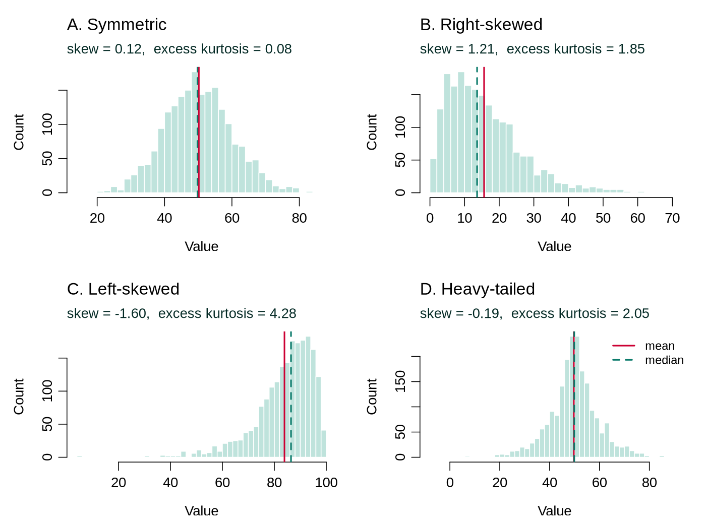
psych::describe() uses. The solid red line is the mean and the dashed line the median: they coincide for symmetric shapes, and the mean is pulled toward the long tail for skewed ones. Panel D has almost no skew but positive excess kurtosis, because both tails are longer than a normal curve would produce.Figure 2.5 shows the link between shape and summary: when the mean and median separate, the distribution is skewed and the median (IQR) is the better summary. In practice the analyst reads the same evidence from R output rather than from a picture.
5.2.4 Reading summary() and describe() Output
Two functions produce most numerical summaries in this course. Base R's summary() gives the minimum, first quartile, median, mean, third quartile and maximum, plus a count of missing values when there are any. The describe() function from the psych package gives a longer row for each variable, including the standard deviation, skew and excess kurtosis. Worked code 2.11 applies both to three variables that Activity 2.3, at the end of this section, does not use.
summary(phaa$diastolic_bp)
library(psych)
describe(phaa[, c("diastolic_bp", "discrimination_score", "social_support_score")])| Column | What it means |
|---|---|
Min., 1st Qu., Median, Mean, 3rd Qu., Max. | For diastolic BP the middle half of readings lies between 64 and 76 mmHg (IQR = 12), and the mean (70.15) and median (70) almost coincide, a sign of a symmetric distribution. A seventh column, NA's, appears when values are missing. |
n | The number of non-missing values. Social support has 780, so 20 values are missing. |
mean, sd, median | The centre and spread that are reported in a results table. |
trimmed, mad | trimmed is the mean after dropping the lowest and highest 10% of values, and mad (median absolute deviation) is the median distance of the values from their median, multiplied by 1.4826 so that it equals the SD for normally distributed data. When they are close to the mean and SD, extreme values have little influence. |
skew, kurtosis | Skewness and excess kurtosis. All three variables have skew between −0.04 and 0.13 and kurtosis between −0.44 and 0.05, so none is noticeably skewed or heavy-tailed. |
se | The standard error of the mean, the SD divided by the square root of n. It describes the precision of the mean; the SD is the measure of spread between people. |
What to report: because the three variables are close to symmetric, each is summarised as mean (SD): diastolic BP 70.2 (9.1) mmHg, discrimination score 7.0 (4.0) and social support score 25.9 (6.0) with 20 values missing. If |skew| were above about 1, or the histogram showed a long tail, the median and IQR from summary() would be reported instead.
The three variables in Worked code 2.11 are all close to symmetric. The worked example below applies the same reading to output in which one variable is strongly skewed and another is an ordered category, which is the situation in which the choice of summary matters most.
Worked Example 2.7: Choosing Summaries From describe() and table() Output
A hospital survey of 640 patients produces the output below for length of stay (days) and a quality-of-life score (possible range 10 to 50), and a frequency table of education. The numbers are hypothetical.
Length of stay. The skew of 2.41 is well above the rule-of-thumb threshold of 1, the excess kurtosis of 7.85 shows much heavier tails than a normal distribution, and the mean (6.8 days) lies far above the median (4.0 days), pulled up by a few very long stays. An SD (7.9) larger than the mean is a further sign of right skew in a variable that cannot fall below zero. Report the median with the IQR (the quartiles come from summary()). A sketch shows a tall peak at short stays, a long tail thinning out to the right towards 58 days, and the median marked to the left of the mean.
Quality of life. The skew (−0.08) is close to 0, the mean (31.4) and median (31.0) almost coincide, and the small negative excess kurtosis (−0.41) means slightly lighter tails and a slightly flatter peak than a normal curve, so the distribution is close to normal. Report the mean and SD, 31.4 (6.2), with the 28 missing values noted. A sketch shows a single, nearly symmetric hump between 12 and 49, centred near 31, with the mean and median at the same point.
Education. The levels are ordered categories, so a mean and SD of the codes have no meaning. Report the count and percentage in each level, in order, among the 600 people with a recorded value (9.7%, 35.7%, 31.2% and 23.5%), and report the 40 missing values. The most common level (the mode) is high school; because the levels are ordered, the median category can also be given, here some college, the level at which the cumulative percentage passes 50%. R gives these numbers directly: round(100 * prop.table(table(dat$education)), 1) prints the percentage in each level among the people with a recorded value, and cumsum() applied to that result prints the cumulative percentages (9.7, 45.3, 76.5 and 100).
The worked example shows that the evidence for a choice of summary sits in the output itself: the skew, the excess kurtosis and the gap between mean and median for a numeric variable, and the variable type for a categorical one. The education row already used a frequency distribution, the main summary for categorical variables, which the next subsection develops.
6.1 Frequency Tables, Cross-Tabulations and the Odds Ratio
For categorical variables, frequency distributions display the count and percentage of observations in each category. Cross-tabulations (contingency tables) display the joint distribution of two categorical variables and are the basis for computing measures of association such as odds ratios and risk ratios. In R, table(x) gives the counts for one variable and table(x, y) cross-tabulates two; prop.table(table(x, y), margin = 1) turns the counts into row proportions, so that each row sums to 1 (100%), and margin = 2 gives column proportions instead. Check which way the percentages run before interpreting them, because the row and column percentages of the same table answer different questions. For example, in a table with smoking status in the rows and hypertension in the columns, row percentages answer "what percentage of smokers have hypertension, compared with non-smokers?", whereas column percentages answer "what percentage of people with hypertension are smokers?" The first compares how common the outcome is in each exposure group, and the second describes who makes up the people with the outcome, so mixing them up leads to a very different conclusion from the same counts.
The most common measure of association from a 2×2 table in epidemiology is the odds ratio. The two worked examples below explain from the start what the number measures. Worked Example 2.8 sets out the cross-tabulation of exposure among cases and controls in an outbreak investigation, shown in Table 2.8, and the odds ratio that R obtains from it.
Worked Example 2.8: Cross-Tabulation in an Outbreak Investigation
Table 2.8. Exposure among 60 cases and 90 controls in an outbreak investigation.
| Cases (n) | Controls (n) | Total | |
|---|---|---|---|
| Exposed | 45 | 30 | 75 |
| Unexposed | 15 | 60 | 75 |
| Total | 60 | 90 | 150 |
Three out of four cases (45 of 60) were exposed, compared with one in three controls (30 of 90). When these four counts are entered in R, as in Worked code 2.12 below, R prints an odds ratio of 6, suggesting a strong association between exposure and disease.
Worked Example 2.8 gives the number; Worked Example 2.9 explains what it measures. It defines odds and shows how the odds ratio is built from them, with the odds of exposure among cases and among controls set out in Table 2.9.
Worked Example 2.9: From Counts to Odds to an Odds Ratio
The odds of a characteristic compare the number of people who have it with the number who do not: odds = number with / number without. For example, 3 people with for every 1 without gives odds of 3, which corresponds to a probability of 0.75 (3 of every 4 people).
In Table 2.8 the four cells are labelled a = 45 (exposed cases), b = 30 (exposed controls), c = 15 (unexposed cases) and d = 60 (unexposed controls).
Table 2.9. Odds of exposure among the cases and the controls of the outbreak investigation.
| Group | Exposed | Unexposed | Odds of exposure (exposed / unexposed) | Odds printed by R |
|---|---|---|---|---|
| Cases | a = 45 | c = 15 | a / c | 3 |
| Controls | b = 30 | d = 60 | b / d | 0.5 |
R prints odds of exposure of 3 among cases and 0.5 among controls (the lines odds_cases and odds_controls in Worked code 2.12): among cases, 3 people were exposed for every 1 who was not, and among controls, 1 person was exposed for every 2 who were not. The odds ratio divides one odds by the other, (a / c) / (b / d), and R prints it as 6. Rearranging gives the cross-product formula, OR = (a × d) / (b × c), which shows that the odds ratio uses all four cells of the table and explains why the same number appears whichever way the ratio is built.
An odds ratio of 1 means the odds are the same in both groups, so there is no association. A value above 1 means the exposure is more common (in odds terms) among cases, and a value below 1 means it is less common. An OR of 6 is a strong association. A descriptive odds ratio makes no allowance for chance or for other differences between the groups; a confidence interval and adjustment for other variables address these.
Together the two worked examples link the number R prints to its meaning: an odds ratio compares the odds of exposure in two groups, and 1 marks no association. In practice the odds and the odds ratio are obtained in R and then interpreted. Worked code 2.12 obtains the outbreak odds ratio in R and applies the same code to hypertension by smoking status in the course data; before reading the result, check which rows and columns of the R table hold the exposed and unexposed cases and controls.
matrix() builds a table from four counts, filling the first column and then the second; dimnames labels the rows and columns. For the course data, table() builds the same kind of table from two variables, and tab["Yes", "No"] picks the cell in the row labelled "Yes" and the column labelled "No".
# The outbreak table from the text
outbreak <- matrix(c(45, 15, 30, 60), nrow = 2,
                   dimnames = list(Exposure = c("Exposed", "Unexposed"),
                                   Group    = c("Case", "Control")))
outbreak
odds_cases    <- outbreak["Exposed", "Case"] / outbreak["Unexposed", "Case"]
odds_controls <- outbreak["Exposed", "Control"] / outbreak["Unexposed", "Control"]
odds_cases
odds_controls
odds_cases / odds_controls              # the odds ratio

# The same steps with the course data: hypertension by smoking status
tab <- table(Smoker = phaa$smoker, Hypertension = phaa$hypertension)
tab
odds_smokers     <- tab["Yes", "Yes"] / tab["Yes", "No"]
odds_non_smokers <- tab["No", "Yes"] / tab["No", "No"]
round(c(smokers = odds_smokers, non_smokers = odds_non_smokers,
OR = odds_smokers / odds_non_smokers), 3)The outbreak calculation reproduces the odds of 3 and 0.5 and the odds ratio of 6. In the course data, 8 of 136 smokers and 15 of 664 non-smokers have hypertension, giving odds of 0.062 and 0.023 and an odds ratio of 2.70: the odds of hypertension are about 2.7 times as high among smokers. With only 23 people with hypertension this estimate is imprecise; a logistic regression would add a confidence interval and adjust for age and other variables.
The course-data example shows that the same two lines of R give the odds ratio for any 2×2 table, provided the cells are read in the right order. A cross-tabulation compares two groups on one characteristic; the next subsection brings many such comparisons together in a single table.
6.2 Constructing a Table 1 Stratified by Exposure
6.2.1 Setting Out a Table 1
In epidemiologic publications, “Table 1” typically presents the baseline characteristics of the study population, often stratified by exposure or outcome status. How baseline characteristics and group comparisons are reported has been the subject of methodological scrutiny. Pocock, Assmann, Enos, & Kasten (2002) reviewed published trial reports and catalogued common problems with baseline comparisons, subgroup analyses and covariate adjustment. A well-constructed Table 1 includes:
- Demographics (age, sex, ethnicity) with appropriate summary statistics
- Key clinical or exposure variables
- Missing data counts for each variable
- A comparison column between groups, preferably standardised differences (explained below)
Setting out the structure of a Table 1 takes three decisions. The columns are the groups being compared, usually the exposure groups (for example, any physical activity versus none), each headed by its number of participants, often with an overall column; the variable that defines the columns is therefore not also a row. The rows are the characteristics that matter for the analysis: demographics, the potential confounders and other covariates, and, if wanted, the outcome. The statistic in each cell follows the reporting convention: mean (SD) for approximately normal continuous variables, median (IQR) for skewed ones, and n (%) for each level of a categorical variable, with the number missing reported for every variable that has gaps.
Table 2.10 shows the structure of a Table 1 for a hypothetical study that compares exposed and unexposed participants. As you read it, check each row's statistic against the reporting convention.
Table 2.10. The structure of a Table 1 for a hypothetical study comparing exposed and unexposed participants, in a layout common in published papers.
| Characteristic | Exposed (n=200) | Unexposed (n=300) | p-value |
|---|---|---|---|
| Age, mean ± SD | 52.3 ± 11.4 | 49.8 ± 12.1 | 0.02 |
| Female, n (%) | 110 (55.0%) | 162 (54.0%) | 0.82 |
| BMI, median (IQR) | 27.1 (24.0–31.5) | 25.8 (23.2–29.4) | 0.004 |
| Current smoker, n (%) | 48 (24.0%) | 51 (17.0%) | 0.05 |
| Diabetes, n (%) | 34 (17.0%) | 30 (10.0%) | 0.02 |
In Table 2.10 the continuous variable with a normal distribution (age) uses mean ± SD, while the skewed variable (BMI) uses median (IQR), and the categorical variables are presented as n (%). In this hypothetical study BMI was right-skewed, so its median (IQR) was reported. In the course data BMI is close to symmetric (skew 0.17 in Activity 2.3), so the course-data table in Worked code 2.13 reports it as mean (SD). The choice follows the distribution of each variable in the data at hand. Table 2.10 also follows a layout common in published papers, with a p-value column and without an overall column or counts of missing values; the course-data table in Worked code 2.13 shows the layout this lesson recommends.
6.2.2 The Comparison Column: p-Values and Standardised Differences
The p-value column of Table 2.10 raises the question of how the groups should be compared. The definitions and the recommendation below are worth committing to memory, because they decide how every Table 1 in this course is read.
Null Hypotheses, p-Values and Standardised Differences
A null hypothesis is the starting assumption of no difference: here, that exposed and unexposed people have the same average age in the population the sample came from. A p-value is the probability of seeing a difference at least as large as the one observed if the null hypothesis were true. A small p-value (conventionally below 0.05) means the observed difference would be surprising if there were truly no difference between the groups.
A standardised difference (also called the standardised mean difference, SMD) expresses the gap between two groups in standard-deviation units. For a continuous variable it is the difference in means divided by the square root of the average of the two groups' variances; for a proportion, the difference in proportions is divided by a standard deviation calculated from the two proportions. An SMD of 0.5 means the groups differ by half a standard deviation. Dividing by a standard deviation puts every variable on the same scale. By this we mean that a difference in age measured in years, a difference in blood pressure measured in mmHg and a difference in the percentage of women can all be compared directly, because each is expressed relative to how much that variable usually varies between people. Values below about 0.1 are commonly read as a negligible imbalance, although this cut-off is a convention.
Recommendation for this course. Table 1 describes the sample, so this course follows the STROBE reporting guideline for observational studies, which advises that significance tests be avoided in descriptive tables (Vandenbroucke et al., 2007). A p-value in Table 1 depends heavily on sample size and describes chance variation; whether an imbalance is large enough to matter as a confounder (a variable that can distort the association between exposure and outcome, defined more fully in 6.2.4) is a separate question, which the standardised difference addresses more directly. Where a comparison column is wanted, report the standardised difference. When a journal requires p-values, they should be read as descriptions of chance variation.
In short, a p-value answers a question about chance that depends on the sample size, whereas a standardised difference measures the size of the imbalance itself. The difference shows up as soon as the sample size changes. For example, the same gap of two years in average age might give a large p-value in a study of 100 people and a very small p-value in a study of 10,000 people, because a larger sample makes it easier to rule out chance. The standardised difference for that gap would be about the same in both studies, because it depends only on the size of the gap relative to the spread of ages, not on how many people were measured. This is why the standardised difference is the better guide to whether an imbalance is large enough to matter.
6.2.3 A Table 1 for the Course Data
Worked code 2.13 puts the three decisions and the standardised difference into practice. It builds a Table 1 for the course data, stratified by smoking status, with an overall column, standardised differences and counts of missing values, and then turns the R output into the report table shown as Table 2.11.
Base R can build Table 1 with three small helper functions. function(v) { ... } defines a reusable recipe, tapply(v, grp, f) applies the recipe f separately to each smoking group, and sprintf() formats numbers as text: %.1f means one decimal place, %d a whole number and %% a percent sign. The comparison phaa$education >= "Bachelor's" works because education was made an ordered factor in the cleaning activity; it is TRUE for a bachelor's or graduate degree.
# Three small helper functions. function(v) { ... } defines a reusable recipe
# that is applied to the whole sample and then to each smoking group.
grp <- phaa$smoker                       # the grouping variable ("No", "Yes")

mean_sd <- function(v) {                 # "mean (SD)" and the standardised difference
  f <- function(x) sprintf("%.1f (%.1f)", mean(x, na.rm = TRUE), sd(x, na.rm = TRUE))
  m <- tapply(v, grp, mean, na.rm = TRUE)
  s <- tapply(v, grp, sd, na.rm = TRUE)
  d <- (m["Yes"] - m["No"]) / sqrt((s["Yes"]^2 + s["No"]^2) / 2)
  c(Overall = f(v), tapply(v, grp, f), SMD = sprintf("%.2f", d))
}
n_pct <- function(v, level) {            # "n (%)" and the standardised difference
  f <- function(x) sprintf("%d (%.1f%%)", sum(x == level, na.rm = TRUE),
                           100 * mean(x == level, na.rm = TRUE))
  p <- tapply(v == level, grp, mean, na.rm = TRUE)
  d <- (p["Yes"] - p["No"]) / sqrt((p["Yes"] * (1 - p["Yes"]) + p["No"] * (1 - p["No"])) / 2)
  c(Overall = f(v), tapply(v, grp, f), SMD = sprintf("%.2f", d))
}
n_miss <- function(v) {                  # number of missing values
  c(Overall = sum(is.na(v)), tapply(is.na(v), grp, sum), SMD = "")
}

table1 <- rbind(
  "N"                     = c(Overall = length(grp), table(grp), SMD = ""),
  "Age, mean (SD)"        = mean_sd(phaa$age),
  "  Age missing, n"      = n_miss(phaa$age),
  "Woman, n (%)"          = n_pct(phaa$gender, "Woman"),
  "Degree, n (%)"         = n_pct(phaa$education >= "Bachelor's", TRUE),
  "BMI, mean (SD)"        = mean_sd(phaa$bmi),
  "SBP, mean (SD)"        = mean_sd(phaa$systolic_bp),
  "Activity, mean (SD)"   = mean_sd(phaa$phys_act_min),
  "  Activity missing, n" = n_miss(phaa$phys_act_min),
  "Income missing, n (%)" = n_pct(is.na(phaa$income), TRUE)
)
noquote(table1)The output has one column for the whole sample, one for non-smokers ("No"), one for smokers ("Yes") and the standardised difference (smokers minus non-smokers). Smokers and non-smokers have nearly the same age (SMD 0.02), proportion of women (0.06), education (−0.09) and physical activity (0.00). Smokers have a lower mean BMI (19.5 versus 21.0 kg/m², SMD −0.50) and a higher mean systolic BP (113.5 versus 107.2 mmHg, SMD 0.56). BMI differs between the groups, but smoking can itself lower body weight, so BMI may be a mediator, a variable on the causal path from smoking to blood pressure. In the simulated course data BMI was generated to depend on smoking status. Adjusting for a mediator removes part of the effect being estimated, so whether BMI enters a model is decided from subject knowledge about causal order, which the regression lessons will need to consider. The missing-value rows show that missing activity data are spread across both groups (20 and 8).
Turning the R output into a report table involves relabelling the columns (with group sizes in the headers), writing units and full names into the row labels, removing the percent signs that the row label already states, and adding a footnote that defines abbreviations. The numbers themselves are copied unchanged, as Table 2.11 shows.
Table 2.11. Characteristics of the course sample, overall and by smoking status, set out for a report.
| Characteristic | Overall (n = 800) | Non-smokers (n = 664) | Smokers (n = 136) | Std. diff. |
|---|---|---|---|---|
| Age (years), mean (SD) | 45.1 (13.6) | 45.1 (13.4) | 45.3 (14.9) | 0.02 |
| Missing, n | 2 | 1 | 1 | |
| Women, n (%) | 414 (51.7) | 340 (51.2) | 74 (54.4) | 0.06 |
| Bachelor's degree or higher, n (%) | 360 (45.0) | 304 (45.8) | 56 (41.2) | −0.09 |
| BMI (kg/m²), mean (SD) | 20.8 (3.2) | 21.0 (3.2) | 19.5 (2.9) | −0.50 |
| Systolic BP (mmHg), mean (SD) | 108.2 (11.3) | 107.2 (11.0) | 113.5 (11.6) | 0.56 |
| Physical activity (min/week), mean (SD) | 176.1 (82.4) | 176.0 (83.4) | 176.1 (77.1) | 0.00 |
| Missing, n | 28 | 20 | 8 | |
| Income not reported, n (%) | 35 (4.4) | 32 (4.8) | 3 (2.2) | −0.14 |
Table note for a report: "Std. diff.: standardised difference, smokers minus non-smokers. SD: standard deviation. BMI: body mass index. One BMI value and two systolic BP values were set to missing by range checks."
Table 2.11 is a complete Table 1: each column is headed by its n, each row carries the statistic that suits it, the missing values are reported, and the comparison column holds standardised differences. A Table 1 stratified by exposure shows how characteristics are distributed across the exposure groups, and the next part explains why that distribution matters before any multivariable model is fitted.
6.2.4 Stratification and Confounding
Stratifying descriptive statistics by key exposure or covariate groups allows you to assess the distribution of potential confounders across exposure categories. By this we mean that each characteristic is summarised separately within each exposure group, so that the groups can be compared side by side, as the columns of Table 2.11 do for smokers and non-smokers. This is a critical step before proceeding to multivariable modelling, as it helps identify imbalances that may require adjustment. If the exposure groups differ on a characteristic that also affects the outcome, a simple comparison of the outcome between the groups mixes the effect of the exposure with the effect of that characteristic.
A confounder is a third variable that is related to both the exposure and the outcome and can therefore make the two appear more, or less, strongly associated than they truly are. Age is a common example, because it is linked to many exposures and to blood pressure. For example, if smokers in a sample were on average much older than non-smokers, smokers would tend to have higher blood pressure partly because of their age, and a crude comparison would overstate the association between smoking and blood pressure. A large standardised difference in Table 1 marks a variable that differs between the exposure groups; whether it also affects the outcome is judged from subject knowledge and the later regression models. A variable that is itself affected by the exposure is a mediator and does not meet the definition of a confounder. The difference lies in causal order. A confounder exists before the exposure and influences both the exposure and the outcome, whereas a mediator comes after the exposure and carries part of its effect to the outcome. Adjusting for a confounder removes a distortion, but adjusting for a mediator removes part of the very effect being estimated.
In the course data, smoking status is the exposure, and the large standardised differences for BMI and systolic BP in Table 2.11 are the variables to think about before any model is fitted. Tables summarise the groups in numbers; the next subsection turns to the plots that show the same data as pictures.
7.1 Choosing a Visualisation
Appropriate visualization depends on the variable type and the question being asked. Exploratory data analysis emphasises looking at data first so structure, gaps, and anomalies are visible before any model is fit. Four kinds of plot cover most needs: a histogram for the shape of one continuous variable, side-by-side boxplots for a continuous variable compared across groups, a bar chart for the frequencies of a categorical variable, and a scatter plot for two continuous variables (or a line graph for a trend over time). Open each tab below to see what each plot shows, when to use it and when not to, with an example from the course data or a simulation.
Histograms display the distribution of a continuous variable by dividing values into bins and counting observations per bin. They reveal distributional shape, modality, gaps, and potential outliers. The choice of bin width affects interpretation: too few bins obscure patterns, too many create noise.
Figure 2.6 shows the same 850 simulated readings, drawn from two groups with different average blood pressures, using 5, 20 and 100 bins. In R the number of bins is suggested with the breaks argument, for example hist(phaa$systolic_bp, breaks = 20); R treats the number as a suggestion and chooses round cut-points near it.
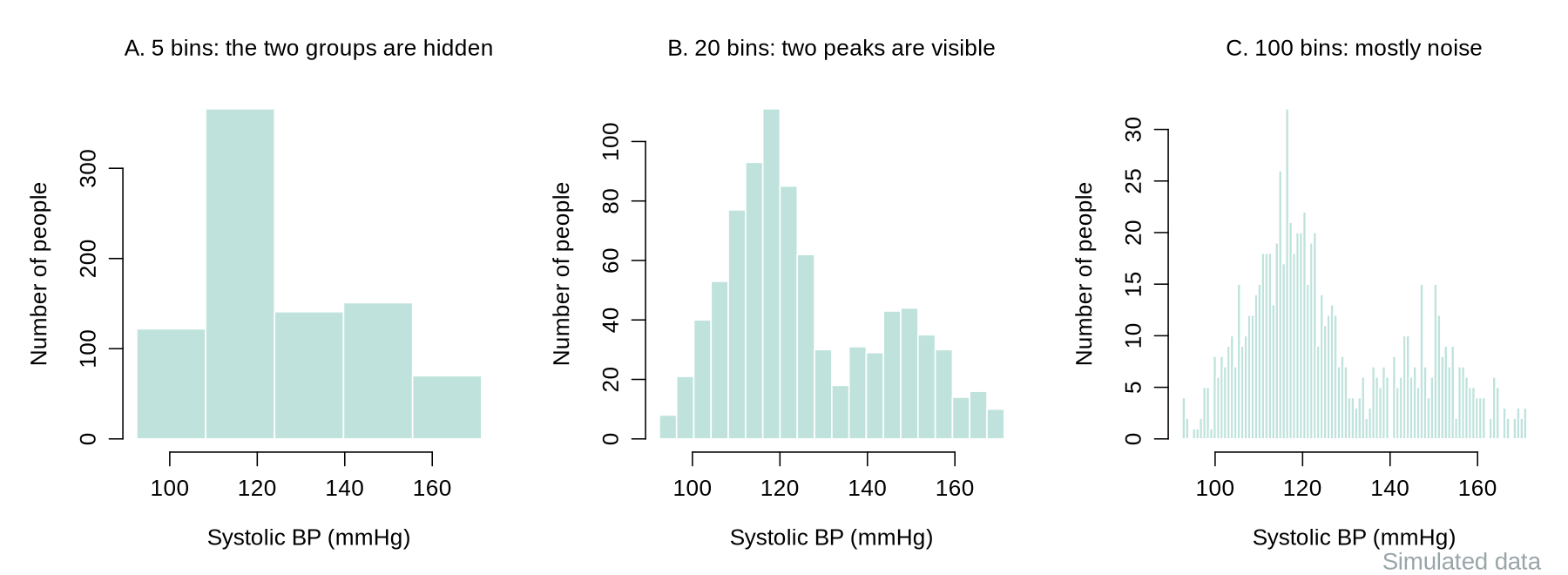
Boxplots display the median, the IQR (the box), whiskers that extend to the most extreme observation lying within 1.5×IQR of the box, and individual points beyond the whiskers. They are ideal for comparing distributions across groups (e.g., blood pressure by treatment arm) and for quickly identifying asymmetry and outliers.
Figure 2.7 shows an annotated boxplot of systolic blood pressure in the course data after the range checks.
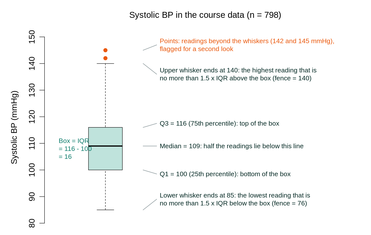
Bar charts display frequencies or proportions for categorical variables. Use them for comparing counts across groups. Avoid using bar charts for continuous data (use histograms instead) and avoid 3D bar charts, which distort proportions.
Scatter plots display the relationship between two continuous variables and can reveal linear or nonlinear associations, clusters, and outliers. Line graphs are appropriate for displaying trends over time (e.g., incidence rates by year). Both are essential in epidemiologic exploratory analysis.
Figure 2.8 plots systolic blood pressure against age in the course data.
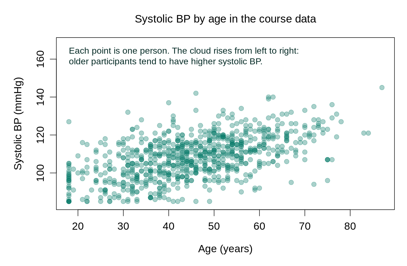
The tabs share one rule: pick the plot by asking what kind of variable you have and what question the picture should answer. A 3D bar chart, or a bar chart of group means, hides the spread and outliers that a group comparison should show. Activity 2.3, at the end of this section, draws the four standard plots described in the tabs for the course data: a histogram, side-by-side boxplots by smoking status, a bar chart and a scatter plot. Always plot before you fit a regression. A boxplot of systolic_bp by smoker tells you in a second whether a regression comparing the two groups will be driven by a few extreme values or by a real shift in the centre of the distribution.
A histogram also gives a first answer to a question that decides which methods are appropriate later: whether a variable is close enough to normal. The next subsection makes that judgement systematic.
7.2 Assessing Normality
7.2.1 Visual Checks and Formal Tests
Assessing whether a variable follows a normal distribution informs the choice between parametric and non-parametric methods. There are two kinds of evidence: visual methods, chiefly the normal Q-Q plot, and formal tests such as the Shapiro-Wilk test. Expand each panel below to see how to read a Q-Q plot and what a test's p-value can and cannot tell you; the caveat about very large samples in the second panel is the point most often missed.
Q-Q (quantile-quantile) plots compare observed quantiles to theoretical normal quantiles. Points falling along the diagonal line suggest normality; systematic departures indicate non-normality. Histograms with a normal curve overlay also provide quick visual assessment.
In plain terms, a Q-Q plot sorts the data from smallest to largest and plots each value against the z-score that a standard normal distribution would place at the same position. These z-scores form the horizontal axis, labelled theoretical quantiles, which runs from about −3 to 3. If the data are normal, the points fall along a straight line. Points that curve away from the line at one end indicate skew, and points that bend away at both ends in an S shape indicate heavy tails, meaning more extreme values than a normal distribution would produce. In R, qqnorm(x) draws the points and qqline(x) adds the reference line.
The Shapiro-Wilk test is generally preferred for samples under 5,000. The Kolmogorov-Smirnov test (with Lilliefors correction) is an alternative. Both test the null hypothesis that data come from a normal distribution.
Because the null hypothesis is normality, a small p-value (below 0.05 by convention) is evidence of a departure from normality, and a large p-value means that no departure was detected. The p-value also depends on sample size: the same small departure gives a large p-value in a sample of 50 and a very small one in a sample of 50,000, because a test with many observations has the power to detect even trivial departures. R's shapiro.test() accepts between 3 and 5,000 values.
Caveat: With very large samples, these tests will reject normality even for trivial departures. Visual assessment should always accompany formal tests.
The three patterns described in the first panel are easiest to learn by sight. Figure 2.9 shows histograms with their normal Q-Q plots for a normal, a right-skewed and a heavy-tailed distribution; compare where each set of points leaves the line.
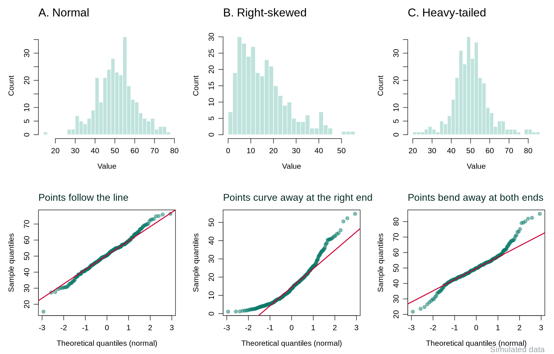
Worked code 2.14 applies both kinds of evidence to the course data: it draws a Q-Q plot of systolic blood pressure and applies the Shapiro-Wilk test to systolic and diastolic blood pressure. Watch how the test result for systolic BP compares with its plot and skew.
qqnorm(phaa$systolic_bp, main = "Systolic BP: normal Q-Q plot")
qqline(phaa$systolic_bp)          # the reference line
shapiro.test(phaa$systolic_bp)
shapiro.test(phaa$diastolic_bp)| Output | What it shows |
|---|---|
W | The test statistic, which is close to 1 when the data look normal. Both values (0.993 and 0.997) are very close to 1. |
| Systolic BP: p-value = 0.0005 | The small p-value means a departure from normality was detected. In the Q-Q plot the points follow the line closely except at the lower end, where the 18 lowest readings are all exactly 85 mmHg and form a short flat run. With 798 readings the test detects this small departure, while the skew of 0.05 shows that the distribution is close to symmetric. |
| Diastolic BP: p-value = 0.10 | No departure from normality was detected. |
Systolic BP shows the large-sample problem at first hand: the test detects a departure (p = 0.0005), yet the plot is close to a straight line and the skew is only 0.05, so the departure is too small to matter.
7.2.2 From the Checks to a Decision
In practice the analyst combines the plot, the skew value and the purpose of the analysis. If the Q-Q plot is close to a straight line and |skew| is below about 1, the variable is summarised as mean (SD) and parametric methods are reasonable, even when a large sample makes the Shapiro-Wilk p-value small, as for systolic BP here. If the plot curves clearly or |skew| is above about 1, the variable is summarised as median (IQR), and the analyst either transforms it (as in the previous section) or uses a rank-based method. Rank-based methods replace each value by its rank (1 for the smallest, 2 for the next, and so on), so a few extreme values cannot dominate the result. Table 2.12 pairs the common options; for each question, read across from the parametric method to its rank-based alternative.
Table 2.12. Parametric and rank-based options for three common analytic questions, with the R function for each.
| Question | Parametric option (assumes approximate normality) | Rank-based option (fewer assumptions) |
|---|---|---|
| Do two groups differ? | The t-test compares the two means: t.test(y ~ group). R uses the Welch version by default, which allows the two groups to have different spreads. | The Wilcoxon rank-sum test compares the ranks of the two groups: wilcox.test(y ~ group). |
| Do three or more groups differ? | One-way analysis of variance (ANOVA) compares the means: summary(aov(y ~ group)). | The Kruskal-Wallis test compares the ranks: kruskal.test(y ~ group). |
| Are two continuous variables associated? | Pearson correlation measures linear association: cor.test(x, y). | Spearman correlation is Pearson correlation calculated on the ranks: cor.test(x, y, method = "spearman"). |
Table 2.12 sums up the decision: if a variable is approximately normal, the parametric methods in the middle column are appropriate, and for clearly non-normal distributions the rank-based alternatives in the right-hand column, or a transformation, are the safer choice. The Central Limit Theorem provides some protection for means in large samples, but descriptive summaries should still reflect the actual distribution. The Central Limit Theorem states that the means of repeated large samples follow an approximately normal distribution even when the individual values do not. By this we mean that a t-test or confidence interval for a mean can still work reasonably well with a skewed variable once the sample is large, because those methods rely on the behaviour of the mean rather than of single values. This protection applies to inference about the mean only. It does not make a skewed variable symmetric, so a Table 1 or a descriptive summary of that variable should still use the median (IQR) when the distribution is clearly skewed.
Additional Context
Building Scales: Internal Consistency and Factor Analysis
This part is background for Activity 2.3 and for analyses that use the depression score, rather than an exam objective. Many public-health surveys ask several items that together measure a latent construct (e.g., depression, anxiety, social support). Two questions need to be answered before you can use these items as a single scale variable in a regression: (1) internal consistency (do the items hang together?), assessed with Cronbach’s α; and (2) dimensionality (how many underlying factors do the items measure?), assessed with exploratory factor analysis (EFA). Once both checks pass, the items can be summed (or averaged) into a derived scale variable that you carry forward into later analyses.
Each depression item asks how often a symptom occurred, on a five-point response scale from 1 (Never) to 5 (Always), so a higher number always means more symptoms. Some questionnaires also include reverse-coded items, worded in the opposite direction (for example, "I felt hopeful about the future"), where a high answer means fewer symptoms. Such items must be flipped before alpha is calculated or a score is built; on a 1 to 5 scale the flipped value is 6 minus the original, so 5 becomes 1 and 1 becomes 5. The alpha() function prints a warning when an item correlates negatively with the rest of the scale, which is the usual sign of an item that has not been reversed. None of the course items is reverse-coded.
Cronbach's alpha can be understood as a measure of how well the items agree. If people who score high on one item tend to score high on the others, the items share a common source, the construct, and alpha is high. Alpha rises when the items are more strongly correlated with each other and when there are more of them. Under the assumptions behind it, an alpha of 0.90 indicates that about 90% of the variation in total scores reflects what the items have in common and about 10% reflects item-specific noise. Values of about 0.70 or higher are conventionally acceptable and 0.80 or higher good; values above about 0.95 can mean that some items are near-duplicates.
Two terms from factor analysis appear in the output. An eigenvalue measures how much of the shared variation among the items one factor accounts for; a large first eigenvalue followed by small ones suggests a single underlying factor. Parallel analysis compares each eigenvalue from the real data with the eigenvalue that random data of the same size would produce, and keeps factors, counting from the first, for as long as the real eigenvalue is larger. A factor loading is the correlation between an item and a factor; loadings of 0.40 or higher are conventionally treated as meaningful, and this lesson uses that threshold throughout.
Activity 2.3, at the end of this section, applies both checks to the seven depression items (dep1 to dep7) and five anxiety items (anx1 to anx5) in the course data: it confirms internal consistency with alpha(), decides on the number of factors with fa.parallel() and factanal(), and builds the derived scale scores. The reference code below prints the full output of these functions for the depression items; the table after it explains each part, and Figure 2.10 annotates the parallel-analysis plot.
# 1. Internal consistency for each candidate scale ----------------------------
library(psych)
dep_items <- phaa[, c("dep1","dep2","dep3","dep4","dep5","dep6","dep7")]
anx_items <- phaa[, c("anx1","anx2","anx3","anx4","anx5")]

alpha(dep_items)             # raw_alpha >= 0.70 is acceptable, >= 0.80 is good
alpha(anx_items)
dep_alpha <- alpha(dep_items)            # store the result to read it at 3 decimals
round(dep_alpha$total$raw_alpha, 3)
round(dep_alpha$alpha.drop[, "raw_alpha", drop = FALSE], 3)  # alpha if an item is dropped

# 2. How many underlying factors? ------------------------------------------
fa.parallel(dep_items, fa = "fa")   # parallel analysis for factors

# 3. Inspect a one-factor solution for the depression items ----------------
factanal(x = na.omit(dep_items), factors = 1)
# na.omit(): factanal() needs complete rows and dep4 has 15 NAs, so these 15
# people are left out of this check (a complete-case analysis).
# With a single factor there is nothing to rotate, so no rotation is requested.
# Loadings >= 0.40 contribute meaningfully to the factor.

# 4. Two-factor solution combining dep + anx items -------------------------
combined <- na.omit(cbind(dep_items, anx_items))
factanal(x = combined, factors = 2, rotation = "varimax")
# dep1-7 should load on one factor; anx1-5 on the other.

# 5. Build derived scale variables for later analyses ------------------------
# Score = mean of the answered items x number of items, calculated only when
# at most one item is missing (otherwise NA). A missing item is never
# counted as 0, which would understate the person's score.
n_dep <- rowSums(!is.na(dep_items))     # items answered by each person
n_anx <- rowSums(!is.na(anx_items))
phaa$dep_score <- ifelse(n_dep >= 6, rowMeans(dep_items, na.rm = TRUE) * 7, NA)
phaa$anx_score <- ifelse(n_anx >= 4, rowMeans(anx_items, na.rm = TRUE) * 5, NA)
summary(phaa$dep_score)| Output | What it shows and what to report |
|---|---|
raw_alpha | Cronbach's alpha, printed to two decimals as 0.9. The line round(dep_alpha$total$raw_alpha, 3) gives 0.904, which is the value to report (α = 0.904). |
std.alpha, average_r | Alpha calculated from standardised items (similar here because all items share the same response scale), and the average correlation between pairs of items (0.57). |
| 95% confidence boundaries | The range of alpha values compatible with the data, 0.89 to 0.91. |
| Reliability if an item is dropped | Each row gives alpha with that item removed. A value above the overall 0.904 would mean the scale is better without the item. Every value here is lower (0.886 to 0.896 at three decimals), so every item contributes; dep7 contributes least, because removing it would lower alpha only to 0.896. |
r.drop (item statistics) | The correlation of each item with the total of the other items, from 0.65 (dep7) to 0.74. Values below about 0.30 would mark an item that does not fit the scale. |
fa.parallel() | The message reports one factor (the number of components is NA because fa = "fa" requests factors only). The annotated plot below (Figure 2.10) shows why. |
factanal() Loadings | All seven loadings lie between 0.691 (dep7) and 0.795 (dep2), well above 0.40. Uniquenesses are the share of each item that the factor does not explain (1 minus the squared loading). |
Proportion Var and the chi-square test | The single factor explains 57.6% of the item variance. The test asks whether one factor is enough; its large p-value (0.551) gives no evidence that more factors are needed. |
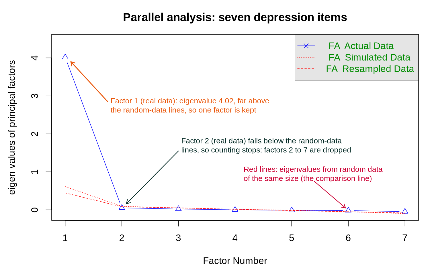
How to read this. An α of 0.904 indicates that the seven depression items measure essentially the same construct. The single factor explains 57.6% of the item variance and every loading is well above the 0.40 threshold (the lowest is 0.691, for dep7), so combining the items into dep_score is justified. Step 5 builds the score as the mean of the answered items multiplied by the number of items (a prorated sum), and only for people who answered at least six of the seven depression items (four of the five anxiety items). Using rowSums(dep_items, na.rm = TRUE) instead would count a skipped item as 0 and understate the scores of the 15 people who skipped dep4, by between 1.8 and 4.5 points (2.8 on average). The score can then serve as a continuous predictor, or as a covariate in a logistic model for hypertension.
Both checks pass for the depression items, so the derived dep_score can be carried forward as a single variable. Activity 2.3 practises everything in this section on the cleaned course data: numeric and categorical summaries, a cross-tabulation and an odds ratio, a Table 1 stratified by smoking status, the four standard plots, a normality check, and the reliability and factor structure of the depression and anxiety items. Run it along with the box and use your own output to answer the questions at the end.
Text version of the activity: the code of the run-along script, its console output and notes on reading it.
phaa <- read.csv("https://heal-learn.ca/r-activities/data/phaa_survey_clean.csv")   # course data, read from the website
phaa$smoker <- factor(phaa$smoker, levels = c("No", "Yes"))
phaa$income <- factor(phaa$income, levels = c("<25k", "25-50k", "50-75k", "75-100k", ">100k"))
library(psych)      # describe(), alpha() and fa.parallel()
library(tableone)   # CreateTableOne() for Table 1
The cleaned file is the survey after the range checks of Section 2, with impossible ages, blood pressures and BMI values set to NA. The income bands are put in order from lowest to highest so that tables list them in that order. If R says that there is no package called psych or tableone, run install.packages(c("psych", "tableone")) once.
summary(phaa$age)
describe(phaa[, c("age", "bmi", "systolic_bp", "phys_act_min")])
table(phaa$income, useNA = "ifany") # ordered categoriesReading the output. For each numeric variable compare the mean with the median and read the skew and the excess kurtosis (0 for a normal distribution). All four are close to symmetric: the largest skew is 0.17 (BMI), far below the rule-of-thumb threshold of 1, and each mean lies within one unit of its median. Physical activity has only 772 values, because some people did not report it. Income is an ordered categorical variable: 50 to 75k is the most common band (207 people), and 35 people did not report income.
round(prop.table(table(phaa$gender, phaa$smoker), margin = 1) * 100, 1)
tab <- table(Smoker = phaa$smoker, Hypertension = phaa$hypertension)
tab
(tab["Yes", "Yes"] / tab["Yes", "No"]) / (tab["No", "Yes"] / tab["No", "No"])With margin = 1 the percentages run along the rows, so each row adds to 100% and shows the share of smokers within each gender: 17.9% of women, 16.4% of men and 11.1% of the 27 non-binary participants (a small, unstable row). In the 2×2 table, 8 smokers and 15 non-smokers have hypertension. Line 22 divides the odds of hypertension among smokers by the odds among non-smokers, both taken from the cells of the table, and prints the odds ratio, 2.70: the odds of hypertension are about 2.7 times as high among smokers. This descriptive odds ratio rests on very few people with hypertension and makes no allowance for chance or for other differences between the groups.
par(mfrow = c(2, 2))
hist(phaa$systolic_bp, main = "Systolic BP", xlab = "mmHg")
boxplot(systolic_bp ~ smoker, data = phaa, ylab = "Systolic BP (mmHg)")
barplot(table(phaa$gender), main = "Gender")
plot(phaa$age, phaa$systolic_bp, xlab = "Age (years)", ylab = "Systolic BP (mmHg)")
par(mfrow = c(1, 1))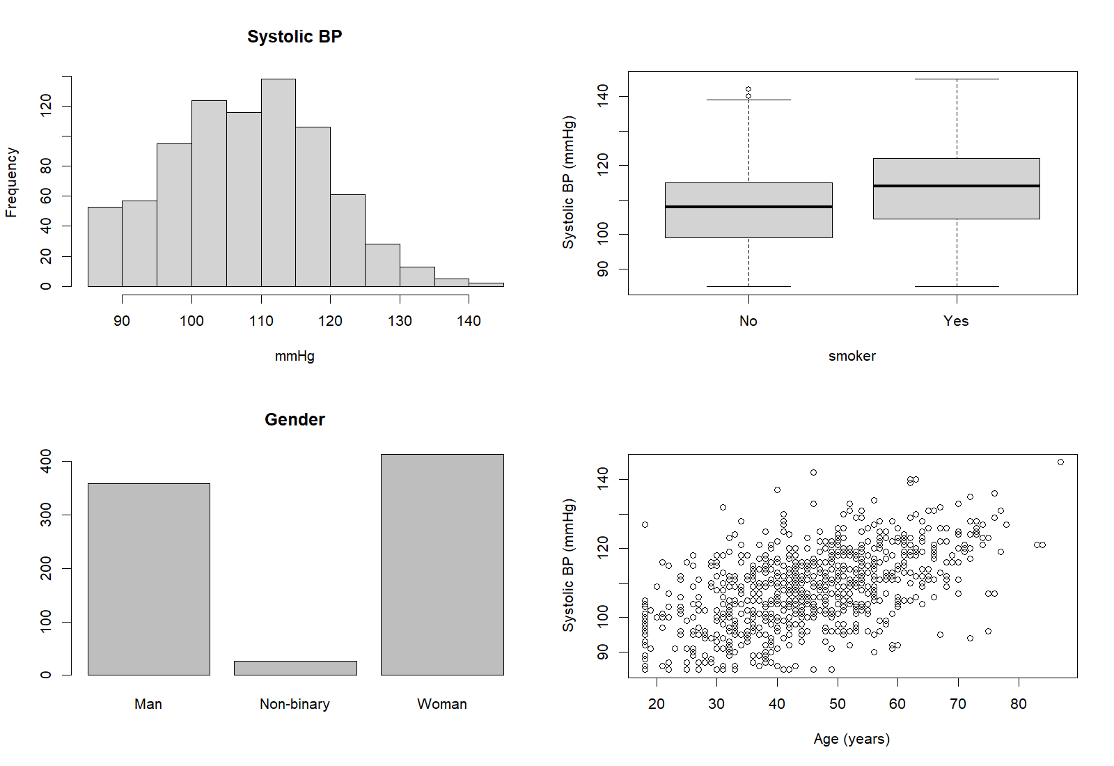
The histogram shows one continuous variable with a single peak near 110 mmHg. The boxplots show a higher median for smokers (114 against 108 mmHg); three non-smoker readings of 140 to 142 mmHg lie beyond the upper whisker, and the smokers have none. The bar chart is for a categorical variable, and the scatter plot shows systolic BP rising with age with no point far from the cloud.
vars <- c("age", "gender", "bmi", "systolic_bp", "phys_act_min", "income")
t1 <- CreateTableOne(vars = vars, strata = "smoker", data = phaa, test = FALSE)
print(t1, smd = TRUE, missing = TRUE)The columns are the exposure groups, non-smokers (664) and smokers (136); smoking defines the columns and is not also a row. Continuous rows show mean (SD) and categorical rows n (%) in each level; print(t1, nonnormal = "...") would show a skewed variable as median [IQR]. The Missing column gives the percentage missing (3.5% for physical activity, 4.4% for income). test = FALSE leaves out p-values; the SMD column gives standardised differences, where values below about 0.1 are read as a negligible imbalance. BMI (0.504) and systolic BP (0.557) differ by about half a standard deviation.
dep_items <- phaa[, paste0("dep", 1:7)]      # dep1 to dep7
anx_items <- phaa[, paste0("anx", 1:5)]      # anx1 to anx5
dep_alpha <- alpha(dep_items)
round(dep_alpha$total$raw_alpha, 3)          # alpha, depression items
round(cbind(dep_alpha$alpha.drop["raw_alpha"], dep_alpha$item.stats["r.drop"]), 3)
round(alpha(anx_items)$total$raw_alpha, 3)   # alpha, anxiety items
fa.parallel(dep_items, fa = "fa")            # how many factors?
factanal(na.omit(dep_items), factors = 1)
combined <- na.omit(cbind(dep_items, anx_items))   # complete rows only
factanal(combined, factors = 2, rotation = "varimax")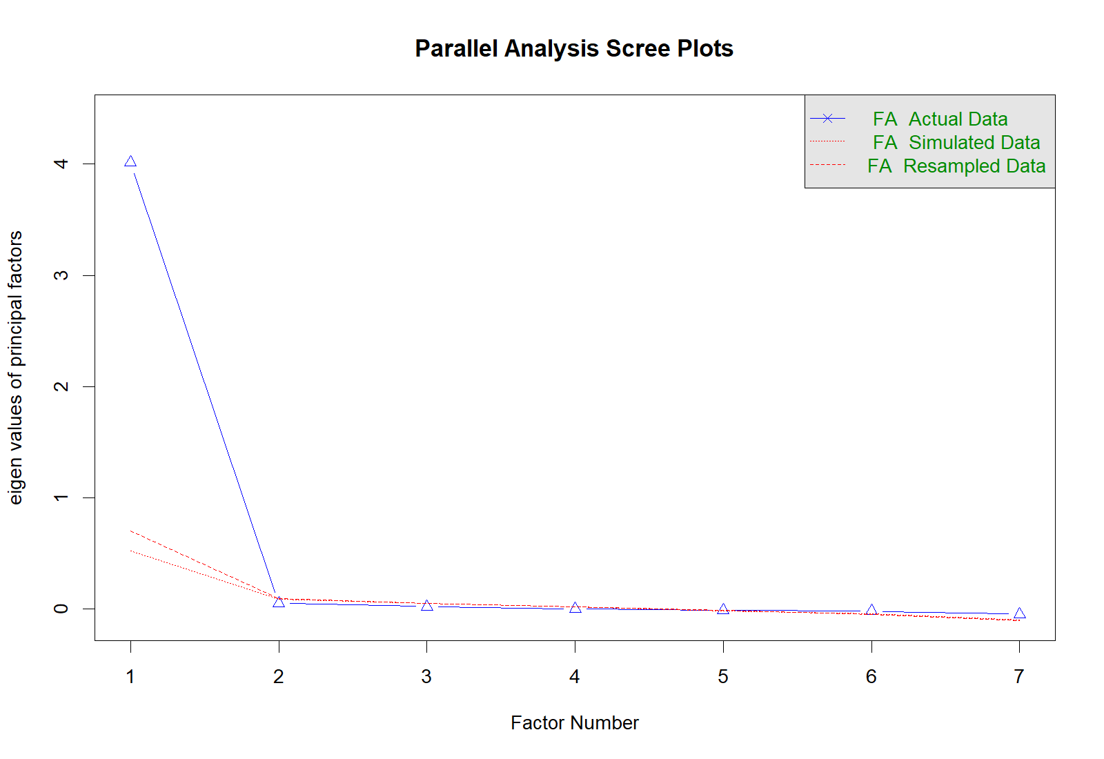
Cronbach's α for the seven depression items is 0.904 (0.80 or higher is good), and for the five anxiety items 0.855. Every alpha-if-dropped value is below 0.904, so every item adds to the scale; dep7 contributes least (0.896 if dropped, item-rest correlation 0.654). Parallel analysis keeps one factor, all seven one-factor loadings lie between 0.691 and 0.795 (well above 0.40), the factor explains 57.6% of the item variance, and the test that one factor is enough gives p = 0.551. In the two-factor solution every depression item loads on Factor 1 and every anxiety item on Factor 2 (own loadings at least 0.68, cross-loadings at most 0.21), so the two scales measure distinct, though related, constructs. na.omit() keeps the complete rows, so the 15 people who skipped dep4 are left out of these checks.
n_dep <- rowSums(!is.na(dep_items))          # items answered by each person
phaa$dep_score <- ifelse(n_dep >= 6, rowMeans(dep_items, na.rm = TRUE) * 7, NA)
n_anx <- rowSums(!is.na(anx_items))
phaa$anx_score <- ifelse(n_anx >= 4, rowMeans(anx_items, na.rm = TRUE) * 5, NA)
summary(phaa$dep_score)Each score is the mean of the answered items multiplied by the number of items (a prorated sum), calculated only for people who answered all but at most one item. A skipped item is never counted as 0: a simple row sum would understate the scores of the 15 people who skipped dep4 by 1.8 to 4.5 points (2.8 on average).
qqnorm(phaa$systolic_bp); qqline(phaa$systolic_bp)
shapiro.test(phaa$systolic_bp)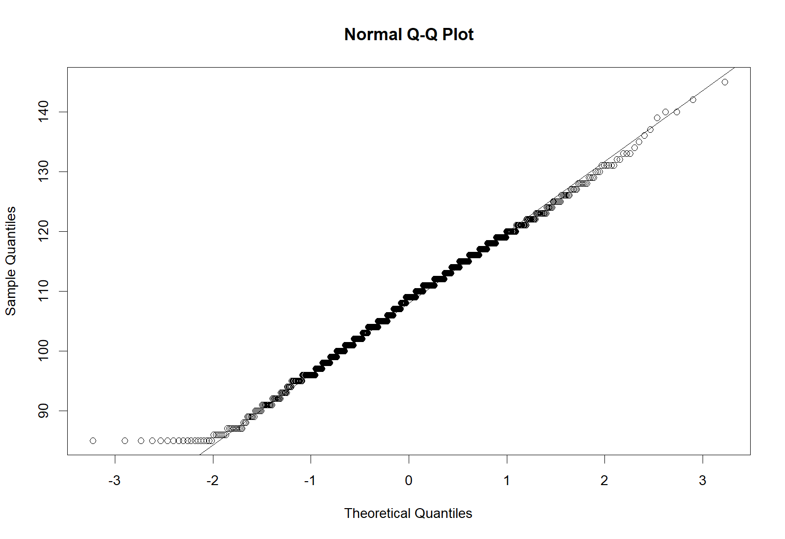
The Q-Q plot follows the reference line closely except at the lower end, where the 18 lowest readings are all exactly 85 mmHg. The Shapiro-Wilk test has normality as its null hypothesis, so p = 0.0005 means that a departure was detected; with 798 readings the test detects even small departures, while the skew of 0.05 shows that the distribution is close to symmetric. The decision rests on the plot and the skew together.
R Reflect on what you just ran
Answer each question from your own output, as on the midterm exam: choose and justify the summaries, set out the table, judge the check.
1. Lines 14 to 16 describe age, BMI, systolic blood pressure and minutes of physical activity a week, and the distribution of household income. For income, type round(100 * prop.table(table(phaa$income)), 1) at the end of the script and run it to print the percentage in each band. For age, systolic BP, physical activity and income, state the measure of central tendency and the measure of spread you would report, and justify each choice with evidence from the output. Then state what the skew and kurtosis of systolic BP indicate about the shape of its distribution and its tails. (describe() reports excess kurtosis, which is 0 for a normal distribution.)
prop.table() line (under 25k 94, or 12.3%; 25 to 50k 159, or 20.8%; 50 to 75k 207, or 27.1%; 75 to 100k 170, or 22.2%; over 100k 135, or 17.6%), with the modal band (50 to 75k) as the typical value and the 35 missing values reported. Income is recorded in ordered categories, so a mean and SD of the bands have no meaning; the spread is shown by the percentage distribution, and because the bands are ordered the median category, 50 to 75k, can also be given. For systolic BP, a skew close to 0 indicates a symmetric distribution, and the small negative excess kurtosis indicates slightly lighter tails and a slightly flatter peak than a normal distribution (mildly platykurtic), so the distribution is close to normal: a single, nearly symmetric hump centred near 108 mmHg, with the mean and median at the same point. A skew above about 1, a mean well above the median, or an SD larger than the mean for a variable that cannot fall below zero would instead call for the median and IQR, because a few extreme values pull the mean and SD towards the long tail.2. Using the output of line 35, set out the structure of a Table 1 for this sample stratified by smoking status: say what the columns are, list the rows you would include and the statistic you would report in each cell, and say how missing values are reported. Then use the SMD column to say which characteristics are balanced between smokers and non-smokers and which differ.
print(t1, nonnormal = ...) produces. Statistic for categorical rows: n (%) in each category, for example 340 (51.2%) and 74 (54.4%) women, with the number missing reported for every variable with gaps (income is missing for 35 people, 4.4%, and physical activity for 28, 3.5%). For the comparison column report the standardised difference (SMD) rather than a p-value, as the STROBE guideline advises, because a p-value depends heavily on sample size; an SMD below about 0.1 is read as a negligible imbalance. Age (0.017), physical activity (0.001) and gender (0.098) are balanced and income (0.118) nearly so, while BMI (0.504; 19.5 against 21.0 kg/m²) and systolic BP (0.557; 113.5 against 107.2 mmHg) differ by about half a standard deviation. BMI may be a mediator, because smoking can lower body weight, so whether a later model adjusts for it is decided from subject knowledge about causal order, not from the table.3. Run your own code: at the end of the script, type shapiro.test(phaa$diastolic_bp) and run it. A colleague notes that shapiro.test(phaa$systolic_bp) gives p = 0.0005 and says that systolic BP must therefore be reported as median (IQR), whereas your output shows that diastolic BP is normal. Do you agree? Explain, using the Q-Q plot from line 57, the skew from line 15 and your own output.
Activity 2.3 turns the cleaned course data into the summaries, tables and plots that a report opens with, and its questions ask you to justify each choice from your own output. This section has described the measures of centre, spread and shape, frequency tables and the odds ratio, the construction of a stratified Table 1, the choice of plots and the assessment of normality, with the construction of scale scores as background. The key takeaways below summarise each of these points, and the knowledge check that follows reviews them.
Key Takeaways
- 5.2 The right summary depends on both the type of variable and the shape of its distribution. For a roughly symmetric continuous variable, report the mean and SD; for a skewed one, report the median and IQR, because a few extreme values pull the mean towards the long tail and inflate the SD; and for categories, report n (%) in each level, with the mode (and, for ordered levels, the median category) as the typical value, never a mean of the codes. To justify your choice from
describe()output, cite the evidence: |skew| above about 1 signals substantial skew, excess kurtosis is 0 for a normal distribution (positive means heavier tails, or leptokurtic; negative means lighter tails, or platykurtic), and a mean well above the median signals a long right tail, as does an SD larger than the mean for a variable that cannot fall below zero. When you sketch the shape the output implies, draw a right-skewed variable as a tall peak at low values with a tail thinning out to the right and the median marked to the left of the mean, and a near-normal variable as a single symmetric hump with the mean and median at the same point. Report the number missing alongside every summary, as the worked example on length of stay, quality of life and education does. - 6.1 A frequency table gives the count and percentage in each category, and a cross-tabulation shows two categorical variables together so that you can compare groups. In R,
table()gives the counts andprop.table(table(x, y), margin = 1)turns them into row proportions, so each row sums to 1 (100%); check which way the percentages run before you interpret them. R gives the odds and the odds ratio from a 2×2 table in a line or two, as in Worked code 2.12, which prints an OR of 2.70 for hypertension by smoking status in the course data. The formula explains what that number is: with a = exposed cases, b = exposed controls (non-cases), c = unexposed cases and d = unexposed controls, OR = (a × d) / (b × c), the odds of exposure among cases divided by the odds among controls (in Worked Example 2.9, an odds ratio of 6.0). An OR of 1 means no association, above 1 means the exposure is more common (in odds terms) among cases and below 1 means it is less common, and a descriptive OR makes no allowance for chance or for other differences between the groups. The most common slip is reading the wrong cells, so check that the rows and columns of the R table match the a, b, c, d layout before you interpret the odds ratio it gives. - 6.2 A Table 1 describes the people in your study before any model is fitted, and stratifying it by exposure shows whether potential confounders are balanced between the groups. Setting it out takes three decisions. The columns are the exposure groups, often with an overall column, each headed by its n, and the variable that defines the columns does not also appear as a row. The rows are the characteristics that matter for the analysis (demographics, potential confounders and other covariates, and the outcome if wanted), and each cell holds the statistic that suits that row: mean (SD) for approximately normal variables, median (IQR) for skewed ones and n (%) for each level of a categorical variable, with the number missing reported for every variable that has gaps. For the comparison column this course follows the STROBE guideline and reports standardised differences rather than p-values, because a p-value depends heavily on sample size; a standardised difference below about 0.1 is commonly read as a negligible imbalance.
- 7.1 Choose a plot by asking what kind of variable you have and what question the picture should answer. A histogram shows the shape of one continuous variable (peaks, tails, gaps and stray clusters, such as readings with a shifted decimal point); try two or three bin numbers, because too few bins can merge two peaks and too many turn the outline into noise. Side-by-side boxplots, such as
boxplot(systolic_bp ~ smoker, data = phaa), compare a continuous variable across groups and show the median, the IQR and the points beyond the 1.5 × IQR fences. Bar charts are for categorical variables only, never for continuous ones; scatter plots show how two continuous variables relate and can reveal a bivariate outlier, such as 191 cm with 46 kg, a combination that is implausible even though each value looks ordinary on its own; and line graphs show trends over time. Plot before you fit any model, because a picture shows in seconds whether a comparison will be driven by a few extreme values or by a real shift in the centre. - 7.2 Before choosing between parametric methods (the t-test, ANOVA, Pearson correlation) and their rank-based alternatives, check whether each continuous variable is close enough to normal. Look at a Q-Q plot (
qqnorm()followed byqqline()), where points along the line suggest normality, points curving away at one end suggest skew and points bending away at both ends in an S shape suggest heavy tails, and look at the histogram and the skew value beside it. A formal test such asshapiro.test()tests the null hypothesis that the data are normal, so a small p-value means a departure was detected, but in a large sample it flags departures too small to matter: systolic BP in the course data gave p = 0.0005 with a skew of only 0.05. Decide from the plot and the skew together: if the plot is close to a straight line and |skew| is below about 1, use mean (SD) and parametric methods; otherwise summarise with median (IQR) and either transform the variable or use a rank-based method (Wilcoxon rank-sum, Kruskal-Wallis or Spearman correlation). - For context: before questionnaire items are combined into a scale score, two checks are needed. Cronbach's α asks whether the items hang together (about 0.70 or higher is acceptable and 0.80 or higher good, as for the seven depression items, with α = 0.904), and factor analysis asks whether they measure one underlying construct (parallel analysis suggests how many factors to keep, and loadings of about 0.40 or more are meaningful). Reverse-coded items must be flipped before either check, and a skipped item should never be counted as 0 when the score is built, because that understates the person's score.
1. A survey of 905 commuters produced the output below for daily commute time in minutes and the Perceived Stress Scale score (possible range 0 to 40). Which choice of summaries and description of shape is correct?
> describe(dat[, c("commute_min", "pss")])
              n  mean    sd median min max  skew kurtosis
commute_min 905 31.60 24.80   24.0   0 165  1.83     4.10
pss         890 18.20  6.10   18.0   2  36  0.05    -0.29
2. A case-control study of a gastrointestinal outbreak at a summer camp asks whether eating from the salad bar was associated with illness. The analyst enters the counts in R and obtains the output below. Which reading of the output is correct?
> salad <- matrix(c(36, 24, 30, 90), nrow = 2,
+   dimnames = list(Salad = c("Ate", "Did not eat"), Group = c("Case", "Control")))
> salad
             Group
Salad         Case Control
  Ate           36      30
  Did not eat   24      90
> odds_cases    <- salad["Ate", "Case"] / salad["Did not eat", "Case"]
> odds_controls <- salad["Ate", "Control"] / salad["Did not eat", "Control"]
> round(c(cases = odds_cases, controls = odds_controls, OR = odds_cases / odds_controls), 3)
   cases controls       OR
   1.500    0.333    4.500
3. An analyst plans four displays for a health survey: (i) the shape of HbA1c values in the whole sample, (ii) BMI compared across four neighbourhoods, (iii) the percentage of respondents in each smoking category, and (iv) whether systolic blood pressure rises with age. Which set of plots matches the variables and the questions?
4. A cohort study compares 420 night-shift workers with 610 day-shift workers. The planned characteristics are age (skew 0.3), alcoholic drinks per week (skew 2.6, with many zeros; missing for 37 people), sex, education (four ordered levels) and current smoking. Which layout for Table 1 follows the conventions taught in this lesson?
5. In a survey of 4,600 adults, diastolic blood pressure has a skew of 0.06, and its normal Q-Q plot follows the reference line closely along its whole length. shapiro.test() gives p = 0.002. What should the analyst conclude?
6. A cross-sectional survey of 480 adults in a rural health region asks whether household food insecurity is associated with type 2 diabetes. The output below describes age and the distance from home to the nearest grocery store (dist_km), and cross-tabulates diabetes by food security. Which set of Table 1 entries, stratified by food security, follows the conventions taught in this section?
> describe(svy[, c("age", "dist_km")])
           n  mean    sd median  min  max skew kurtosis
age      480 47.80 13.20   47.0 19.0 84.0 0.18    -0.40
dist_km  466  6.90  8.40    3.9  0.2 52.5 2.64     8.31
> quantile(svy$dist_km, c(0.25, 0.75), na.rm = TRUE)
25% 75%
1.8 8.6
> sum(is.na(svy$dist_km))
[1] 14
> tab <- table(svy$food_insec, svy$diabetes)
> tab

            no yes
  secure   288  32
  insecure 120  40
> rowSums(tab)
  secure insecure
     320      160
> round(100 * prop.table(tab, margin = 1), 1)

           no yes
  secure   90  10
  insecure 75  25
rowSums()), so food security is not also a row. The statistic in each row follows the variable's type and shape: age is close to symmetric (skew 0.18, excess kurtosis −0.40, mean 47.8 against median 47.0), so mean (SD); distance is strongly right-skewed (skew 2.64, excess kurtosis 8.31, mean 6.9 against median 3.9 km, and an SD larger than the mean), so median (IQR), with the 14 missing values reported; and diabetes is categorical, so n (%) from the row percentages, 10% and 25%. Option (b) is tempting because the sample is large, but a large sample does not make a skewed variable symmetric, and a categorical variable is reported as n (%); option (a) reverses the two continuous rows and repeats the exposure as a row; and option (c) gives up the stratification that shows whether characteristics are balanced between the groups. (Section 3, 5.2.2 Measures of Spread, reporting convention, Worked Example 2.7, 6.1 Frequency Tables, Cross-Tabulations and the Odds Ratio and 6.2.1 Setting Out a Table 1; Objectives 5.2 and 6.2)● Complete the knowledge check to continue.
Final Assessment
Bringing It All Together
This lesson followed a single dataset from raw to descriptive. The section on data quality named the errors (collection, entry, storage, and analysis-stage problems) and unpacked the missing-data mechanisms (MCAR, MAR, MNAR) that determine which cleaning approaches are valid. The section on cleaning strategies turned that vocabulary into a workflow: systematic range, type, and consistency checks; outlier triage; principled missing-data handling; transformations and derived variables; and a documentation trail that a peer reviewer could follow. The section on descriptive analyses closed the loop with the layer that every paper opens with: central tendency, spread, shape, frequency tables, visualisations, scale checks, and a Table 1 that stratifies on the primary exposure or outcome.
Descriptive analysis is a core stage of any analysis. It is the layer where data problems surface, where assumptions get tested, and where readers calibrate how much trust to place in the inferential models that follow. Regression models can then be fitted knowing that the dataset under them has been examined and understood.
Key Takeaways from this lesson
- You can now read a few raw rows beside a data dictionary, name the errors and coding faults you see (transcription, coding, logical inconsistency, out-of-range and duplicate errors; missing codes that could be real values, compound codes, text in numeric fields, mixed date formats and inconsistent missing values), say where in the pipeline each one entered, and state how to correct it. For each fault, give both halves of the answer, the problem and its best-practice correction, and remember that every correction is made in a script that reads the raw file, never by editing the raw file by hand.
- You can classify a described pattern of missing data as MCAR, MAR or MNAR by asking what the missingness depends on: nothing about the people, observed variables only, or the missing value itself. Answer in three parts every time: the label, a one-sentence justification that names what the missingness depends on, and the consequence of a complete-case analysis (unbiased but less precise under MCAR, possibly biased under MAR, and biased under MNAR in a way that imputation under the MAR assumption does not correct).
- You can run range, type, consistency and outlier checks, decide whether each flagged value should be kept, transformed or excluded, and write the rule in a cleaning log. In a question built on R output, compare the Min. and Max. from
summary()with the documented valid range, set impossible or miscoded values toNAwhile keeping the row, and never choose a transformation to fix an error; then write a rule that names the variable, the limit broken, the action, the number of values affected, and who made the change and when. - You can choose a missing-data method that suits the plausible mechanism and the amount missing: complete-case analysis when little is missing and MCAR is plausible, and multiple imputation pooled with Rubin's rules under a stated MAR assumption otherwise. Remember that single imputation treats guessed values as known, which makes standard errors too small, and that the share of rows an analysis loses can be much larger than the share missing on any one variable.
- You can choose, obtain in R and interpret the measures of centre, spread and shape that suit each variable's type and distribution, and sketch the shape a summary implies. When you justify a choice from
describe()output, cite the evidence: |skew| above about 1, excess kurtosis well away from 0 and a mean far from the median point to the median (IQR); skew and excess kurtosis near 0 with the mean close to the median point to the mean (SD); and categorical variables are summarised as n (%) with the number missing reported. - You can build frequency tables and cross-tabulations, obtain in R and interpret an odds ratio from a 2×2 table, and set out a Table 1 stratified by exposure. Check which cells of the R table are a, b, c and d, the cells in OR = (a × d) / (b × c), before you interpret the odds ratio that R prints, and in a Table 1 head each exposure column with its n, choose the statistic row by row, report the missing values, and leave the exposure itself out of the rows.
- You can choose a plot that suits the variable and the question, and judge whether a variable is close enough to normal for parametric methods. Base that judgement on a Q-Q plot, a histogram and the skew together rather than on a Shapiro-Wilk p-value alone, because in large samples the test flags departures too small to matter; when the shape is clearly non-normal, transform the variable or use a rank-based method.
Final Knowledge Assessment
You must answer all 16 questions correctly (100%) to finish this lesson.
1. One participant's record shows smoking status "Never smoked" and cigarettes per day = 15. Each value lies within its valid range in the data dictionary. What type of error is this, and which check would find it?
2. A clinic sends the raw extract and data dictionary below. Which pair of corrections follows best practice?
id   n_visits  first_visit
A01  3         2024-11-05
A02  none      05/11/2024
A03  1         5 Nov 24

Data dictionary as supplied
  n_visits     number of clinic visits in 2024
  first_visit  date of first visit
3. In a survey of 1,200 university students, the item on alcoholic drinks per week is missing for 9%. Follow-up interviews suggest that the heaviest drinkers were the most likely to skip the item, and no recorded variable explains who skipped it. Which classification and consequence are correct?
4. Household income is missing for 12% of 3,000 survey respondents. Respondents without an income value are on average 9 years older than those with one, and age is recorded for everyone. A colleague writes: "The mechanism cannot be checked, so we will assume MCAR and analyse complete cases, which gives unbiased estimates." What is the best response?
5. A study of 900 participants analyses four variables. Because a printing fault skipped one page in a random set of questionnaires, 14 participants (1.6%) lack a value on one of the four variables; nothing else is missing. Which approach is defensible?
6. The first cleaning pass of a cardiology survey prints the output below. The codebook gives hard limits of 30 to 220 beats per minute for resting heart rate (hr_rest). What should be done with the affected values?
> summary(dat$hr_rest)
   Min. 1st Qu.  Median    Mean 3rd Qu.    Max.
  41.0    62.0    69.0    70.4    77.0   720.0
> sum(dat$hr_rest > 220)
[1] 2
7. Waist circumference in a sample has a mean of 92 cm and an SD of 13 cm. The analyst converts two readings, 135 cm and 60 cm, to z-scores in R. Using the z-score rule, which statement is correct?
> round((c(135, 60) - 92) / 13, 2)   # z = (x - mean) / SD
[1]  3.31 -2.46
8. A colleague found 14 systolic readings of 1,100 to 1,500 mmHg, each with a shifted decimal point. She opened the raw spreadsheet, typed the corrected values (110 to 150 mmHg) over them, and saved the file under its original name. What is the main problem, and what should she have done?
9. Self-rated health was recorded in five ordered levels, and R gives the output below. How should the variable be summarised?
> table(dat$srh, useNA = "ifany")
     Poor      Fair      Good Very good Excellent      <NA>
       48       152       410       290       100        50
> pct <- round(100 * prop.table(table(dat$srh)), 1)   # among the 1,000 with a value
> pct
     Poor      Fair      Good Very good Excellent
      4.8      15.2      41.0      29.0      10.0
> cumsum(pct)                                          # cumulative percentages
     Poor      Fair      Good Very good Excellent
      4.8      20.0      61.0      90.0     100.0
prop.table() gives the percentage in each level among the 1,000 recorded values, and the cumulative percentage first passes 50% at "Good" (61.0%), so the median category is "Good", which is also the most common level (the mode). Option (d) is tempting because percentages of the recorded values are correct, but the 50 missing values must still be reported. (Section 3, 5.2.4 Reading summary() and describe() Output, Worked Example 2.7; Objective 5.2)10. Five participants report 4, 6, 8, 10 and 12 hours of moderate activity per week, and R gives the output below. Which statement reads it correctly?
> hrs <- c(4, 6, 8, 10, 12)
> mean(hrs)
[1] 8
> var(hrs)   # the variance
[1] 10
> sd(hrs)    # the standard deviation
[1] 3.162278
11. The output below describes age at death (years) in a regional death registry. Which reading is correct?
> describe(dat["age_death"])
             n  mean    sd median min max  skew kurtosis
age_death 2140  76.1  12.4   79.0  22 104 -1.35     2.20
describe() reports excess kurtosis, for which 0 is the value for a normal distribution, so 2.20 means heavier tails (leptokurtic). Option (c) is the common mistake of comparing the value with 3, which applies only to kurtosis before 3 is subtracted. With substantial skew, the median and IQR describe a typical age at death better than the mean and SD. (Section 3, 5.2.3 Measures of Shape, Skewness and Kurtosis panels; Objective 5.2)12. A case-control study of hip fracture in adults over 70 recorded regular exercise. Among 80 cases, 20 exercised regularly and 60 did not; among 160 controls, 64 exercised regularly and 96 did not. The analyst obtains the odds ratio in R. What does the output show?
> hip <- matrix(c(20, 60, 64, 96), nrow = 2,
+   dimnames = list(Exercise = c("Regular", "Not regular"), Group = c("Case", "Control")))
> hip
             Group
Exercise      Case Control
  Regular       20      64
  Not regular   60      96
> odds_cases    <- hip["Regular", "Case"] / hip["Not regular", "Case"]
> odds_controls <- hip["Regular", "Control"] / hip["Not regular", "Control"]
> round(c(cases = odds_cases, controls = odds_controls, OR = odds_cases / odds_controls), 3)
   cases controls       OR
   0.333    0.667    0.500
13. A cohort study enrolled 3,000 e-cigarette users and 3,000 non-users. Its Table 1 reports age, mean (SD), as 41.2 (12.0) in users and 35.8 (11.8) in non-users (standardised difference 0.45, p < 0.001), and women as 51.5% of users and 48.5% of non-users (standardised difference 0.06, p = 0.02). Which interpretation is correct?
14. Hospital charges were recorded for 70 patients, 35 on each of two wards. The normal Q-Q plot curves upward away from the line at the right end, the skew is 2.2 and shapiro.test() gives p < 0.001. The analyst wants to compare the two wards. Which plan is most appropriate?
15. An analyst wants to see whether a few extreme values drive the differences in systolic blood pressure between three clinics. She plans a 3D bar chart of the three clinic means. Which display should she use instead?
16. In a diabetes education programme with 412 participants, HbA1c at the six-month follow-up is missing for 62 (15%), almost all in the evening session (recorded in the file as session), because the laboratory closed early on evening-session days. Evening participants are younger and more often employed than daytime participants, and within each session, whether the value is missing is unrelated to the participant's HbA1c. A colleague says the values are missing completely at random, "because a laboratory closing early has nothing to do with the participants", and plans a complete-case analysis. What is the best response?
✦ Before submitting: pass every section knowledge check (100%).