n
0
Exploratory Data Analysis For Epidemiology
lm().glm(family = binomial) through its odds ratios and predicted probabilities.This course was developed by Dr. Kiffer G. Card based on Dohoo, I. R., Martin, S. W., & Stryhn, H. (2012). Methods in Epidemiologic Research. VER Inc.
📚 Reference page, available throughout the lesson
This glossary collects the key concepts, methods and people in this lesson. It can be used as a reference while working through the material or as a review before assessments. Typing in the search box filters the entries.
lm().
predict(model, newdata, type = "response").
age:smoker, together with both main effects.
lm().
plot(model) draws four diagnostic plots: residuals versus fitted values, a Q-Q plot of the residuals, a scale-location plot and residuals versus leverage.
bptest()) checks equal variance, and the Shapiro-Wilk test (shapiro.test()) checks normality of the residuals. Both become very sensitive in large samples.
coeftest(model, vcov = vcovHC(model, type = "HC3")).
glm(..., family = binomial).
This section begins with the familiar tests that compare two variables at a time and then introduces regression, which compares many variables at once. It explains how to choose a two-variable test from the types of the two variables, and which rank-based or exact test replaces it when an outcome is skewed or ordinal or when counts are small; how to read the result of each test from R; and why a third variable can distort a two-variable comparison. It then describes the regression line and least squares, shows that the simple tests are special cases of regression, and explains why each coefficient in a model with several predictors is an adjusted estimate. All of the examples use phaa_survey_clean.csv, the cleaned PHAA survey of 800 adults, with systolic blood pressure as the main outcome.
A two-variable test asks whether two variables are associated. The choice of test depends on the type of each variable, which is either numeric (continuous or discrete) or categorical (binary, nominal or ordinal). The type follows from what a variable means rather than from how it is stored: a rating stored as the numbers 1 to 5 is still ordinal, and a variable coded 0 and 1 is still categorical. Table 3.1 lists the four tests used most often in this course, with the result of each in the PHAA survey.
Table 3.1. The four two-variable tests used most often in this course, with the R function for each and an example of its result in the PHAA survey.
| Outcome | Predictor | Test and R function | Example in the PHAA data | Result |
|---|---|---|---|---|
| Numeric | Numeric | Pearson correlation, cor.test() | Systolic BP and age | r = 0.54 (95% CI 0.49 to 0.59), p < 0.001 |
| Numeric | Two groups | Two-sample t-test, t.test() | Systolic BP by smoking | Difference 6.3 mmHg (4.2 to 8.4), p < 0.001 |
| Numeric | Three or more groups | One-way ANOVA, aov() | Systolic BP by region | F = 1.74 on 4 and 793 df, p = 0.14 |
| Categorical | Categorical | Chi-square test, chisq.test() | Elevated BP by smoking | 12.1% against 35.6%, χ² = 44.2, p < 0.001 |
Each test has its own assumptions, that is, conditions that the data must roughly meet for the p-value and confidence interval to be trustworthy. The correlation coefficient measures a straight-line relationship, so a strong but curved relationship can produce a small correlation. The t-test and ANOVA assume roughly normal outcomes within each group (or reasonably large groups), and the classic versions assume similar spread in each group; R's default t.test() uses the Welch version, which does not require equal spread, and var.equal = TRUE requests the classic version used in this section. The chi-square test needs an expected count of about 5 or more in each cell of the table. When these assumptions are doubtful, a rank-based or exact version of the test is used instead, as 1.1.2 describes.
The chi-square row of Table 3.1 needs a categorical outcome, whereas systolic blood pressure is numeric. Worked Example 3.1 applies the variable-type rule to that row: it shows how blood pressure is recoded as a yes-or-no variable and what the recoding costs.
The chi-square test needs two categorical variables, so systolic blood pressure is recoded as elevated (120 mmHg or more) or not. In R this takes one line, phaa$elevated_bp <- factor(ifelse(phaa$systolic_bp >= 120, "Yes", "No"), levels = c("No", "Yes")), which gives 128 people with elevated blood pressure and 670 without (2 readings are missing). Recoding a continuous variable throws away information, because a reading of 121 and a reading of 145 become the same category, so it is done only when a yes-or-no outcome answers the question being asked. The survey's own hypertension variable has only 23 cases, too few for the multivariable models in Section 3, which is why this lesson uses elevated blood pressure as its yes-or-no outcome.
The recoded variable makes the chi-square comparison possible, and it returns as the outcome of the logistic models in Section 3.
The tests in Table 3.1 rely on assumptions about the data, and two families of backup tests exist for situations in which those assumptions are doubtful. A rank-based (non-parametric) test replaces each value with its position in the sorted data. By this we mean that the smallest value becomes rank 1, the next smallest becomes rank 2, and so on, and the test is then carried out on these ranks rather than on the original values. Because a rank records only the order of the values and not their distance from one another, a few extreme values carry little weight. For example, the highest blood pressure reading in a sample receives the top rank whether it lies 5 mmHg or 50 mmHg above the next reading, so one unusually high reading cannot drag the result in the way it can drag a mean. An exact test works differently. Instead of relying on an approximation that is accurate only when the sample is reasonably large, as the chi-square test does, it calculates its p-value directly from every possible arrangement of the data that is consistent with the observed totals. As a result, an exact test remains accurate in small samples, where an approximate test can give a misleading p-value.
When the assumptions of a test look doubtful, use its rank-based version (Spearman’s ρ, the Mann–Whitney U test, the Wilcoxon signed-rank test for paired data, or the Kruskal–Wallis test) when the outcome is skewed or ordinal, and Fisher’s exact test when an expected count in a 2 × 2 table falls below about 5. Before naming any test, also check whether the groups are independent or paired.
Many of the familiar two-variable tests are special cases of the general linear model, the family that includes linear regression and analysis of variance, so the regression models of this lesson can carry out the same comparisons. The simpler tests nonetheless remain in wide use. They are the conventional way to report crude comparisons, such as the group differences in a descriptive “Table 1”, where no adjustment is intended. They are familiar to readers, report the comparison directly in the units of the question, and require fewer modelling decisions, and their rank-based and exact versions accommodate skewed distributions, ordinal scales, and small samples.
Table 3.2 lists the basic tests, the R function that runs each one, and the regression model that returns the same or a closely related result. Where a rank-based test is listed, it is chosen because of the shape of the distribution or the measurement scale, and a histogram or a normal Q-Q plot of the variable shows whether its distribution is close enough to normal.
Table 3.2. The R function and the regression counterpart of each basic two-variable test, including the rank-based and exact versions.
| Test | Compares | R function (example) | Regression counterpart |
|---|---|---|---|
| Pearson correlation | Linear association between two continuous variables | cor.test(x, y) | lm(y ~ x); the slope test gives the same t and p-value |
| Spearman’s ρ (rank-based) | Monotonic association when either variable is skewed or ordinal | cor.test(x, y, method = "spearman") | The same coefficient as a Pearson correlation of the ranks, cor(rank(x), rank(y)) |
| Two-sample t-test | Means of a continuous outcome in two independent groups | t.test(y ~ group) | lm(y ~ group); the same p-value as t.test(y ~ group, var.equal = TRUE), with the sign of t reversed (R’s default Welch test differs slightly) |
| Paired t-test | The mean within-pair difference, as in before-and-after measurements | t.test(after, before, paired = TRUE) | lm(I(after - before) ~ 1); the intercept test is identical |
| Mann–Whitney U (Wilcoxon rank-sum, rank-based) | Two independent groups when the outcome is skewed or ordinal | wilcox.test(y ~ group) | Closely approximated by lm(rank(y) ~ group) |
| Wilcoxon signed-rank (rank-based) | Within-pair differences that are skewed or ordinal | wilcox.test( | Closely approximated by an intercept-only regression on the signed ranks of the differences |
| One-way ANOVA | Means of a continuous outcome across three or more groups | summary(aov(y ~ group)) | lm(y ~ group); the same F-test |
| Kruskal–Wallis (rank-based) | Three or more groups when the outcome is skewed or ordinal | kruskal.test(y ~ group) | Computed from a one-way ANOVA on the ranks, lm(rank(y) ~ group) |
| Pearson χ² | Association between two categorical variables | chisq.test( | glm(y ~ x, family = binomial); for a 2 × 2 table its score test, anova(fit, test = "Rao"), equals χ² computed with correct = FALSE, that is, without the continuity correction, a small adjustment that R applies to 2 × 2 tables by default |
| Fisher’s exact test (exact) | A 2 × 2 table with small expected counts | fisher.test( | Exact logistic regression, a version of logistic regression for small samples that this course does not develop |
| McNemar’s test | Paired binary outcomes, as in matched pairs or before-and-after measurements | mcnemar.test( | Conditional logistic regression, a version of logistic regression for matched data that this course does not develop; its score test equals McNemar’s χ² computed with correct = FALSE |
| Cochran–Armitage trend test | A binary outcome across ordered categories | prop.trend.test( | glm(y ~ score, family = binomial); its score test is the same statistic |
The last column of Table 3.2 shows that each test has a regression counterpart, a point that 2.2 develops. Choosing the test is the first step; the next is to run it in R and read its result.
Each test in Table 3.1 is run with one line of R, and Activity 3.1 at the end of this section runs all four on the PHAA survey. Reading the result is where the marks lie. For every test, report the estimate in the units of the question (a correlation, a difference in means, or the two percentages being compared), its 95% confidence interval and its p-value, and then say in plain words what they mean.
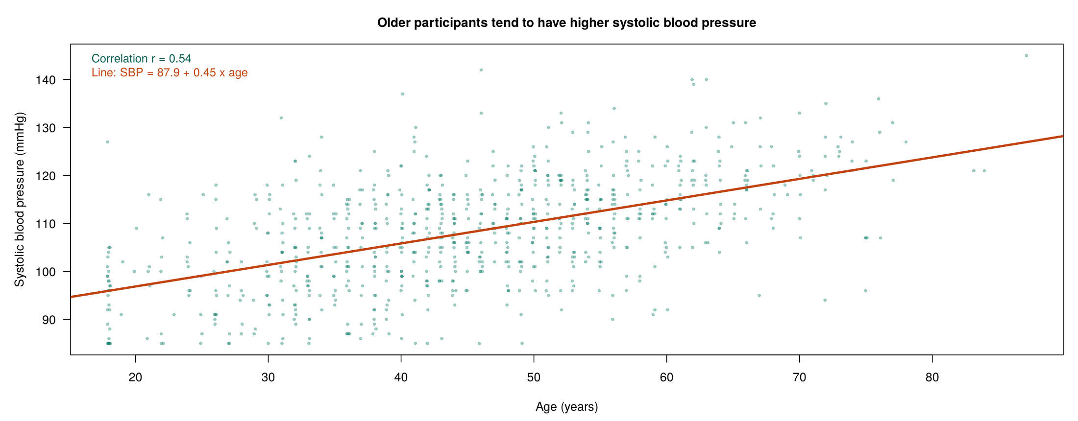
In the PHAA survey, the correlation between age and systolic blood pressure is 0.54 (95% CI 0.49 to 0.59), a moderate positive association in which older participants tend to have higher blood pressure. Smokers average 6.3 mmHg higher than non-smokers (95% CI 4.2 to 8.4 mmHg, p < 0.001). The mean blood pressure of the five regions ranges only from 106.1 to 109.1 mmHg, and the ANOVA gives p = 0.14, so the regional differences are consistent with chance. Elevated blood pressure is present in 35.6% of smokers and 12.1% of non-smokers (χ² = 44.2, p < 0.001), a clear association.
Each of the three reported quantities answers a different question. The estimate gives the size of the association, such as the 6.3 mmHg difference between smokers and non-smokers. The confidence interval gives the range of population values that are consistent with the data. By this we mean that the sample is only one of many that could have been drawn, and the interval shows how far the true population difference could plausibly lie from the sample estimate. The interval and the p-value are linked: an interval for a difference that lies entirely above or below 0 goes with a p-value below 0.05, because 0, the value that would mean no difference, is then not among the plausible values.
The p-value is the probability of a difference at least as large as the one observed if there were no difference in the population. In other words, it asks how surprising the data would be in a world where the null hypothesis of no difference is true. Because it is calculated by assuming that there is no difference, it cannot also be the probability that the null hypothesis is true. In addition, on its own it says nothing about the size of the effect: a very large sample can give a tiny p-value for a difference too small to matter, and a small sample can give a large p-value for a difference that is important. A two-variable comparison also describes groups on average. A difference in means is not a fixed change in every person, since some smokers have lower blood pressure than some non-smokers. Nor does it show cause, because the groups may differ in other ways, such as age, that also affect the outcome.
One detail of the R output needs care. t.test(systolic_bp ~ smoker, data = phaa, var.equal = TRUE) subtracts the second group (smokers) from the first (non-smokers), so it prints the 95% interval as −8.35 to −4.24 mmHg, which is reported as smokers being between 4.24 and 8.35 mmHg higher. For a chi-square test, chisq.test(tab)$expected prints the expected counts that the rule of about 5 per cell refers to, and R warns that the chi-square approximation may be incorrect when any of them is too small. These results describe how two variables go together, but not why, and the next subsection shows how a third variable can distort such a comparison.
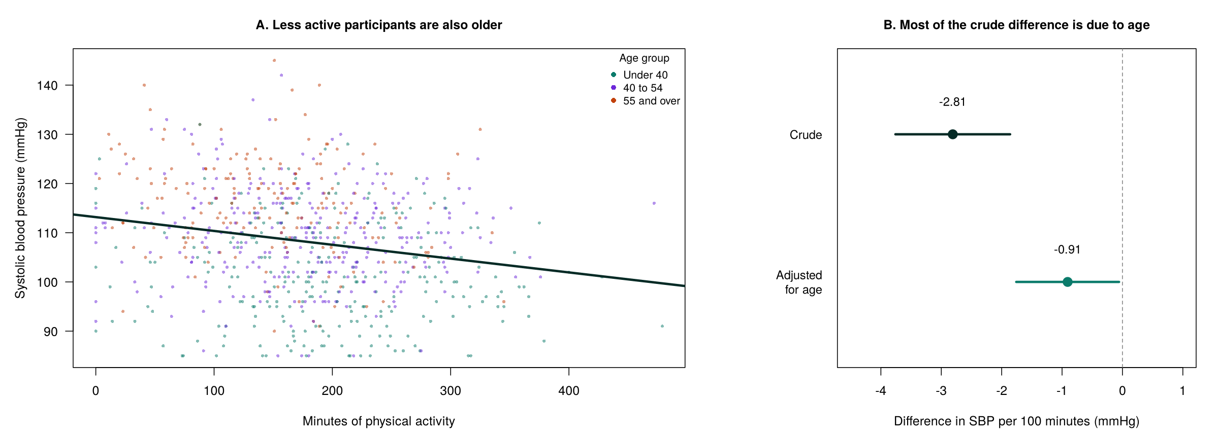
A two-variable test compares people who differ in the predictor, but those people may also differ in many other ways. When a third variable is related to both the predictor and the outcome, it can create, hide or exaggerate an association. Such a variable is called a confounder. By this we mean a variable that travels alongside the predictor, so that part of the difference attributed to the predictor is really a difference in the confounder. For example, if the people who exercise more are also younger, and younger people have lower blood pressure, then active people will have lower blood pressure even if exercise itself had no effect at all. Because the two-variable test sees only exercise and blood pressure, it has no way to separate the part of the difference that belongs to exercise from the part that belongs to age. Figure 3.1 illustrates this with physical activity and systolic blood pressure, where age is related to both.
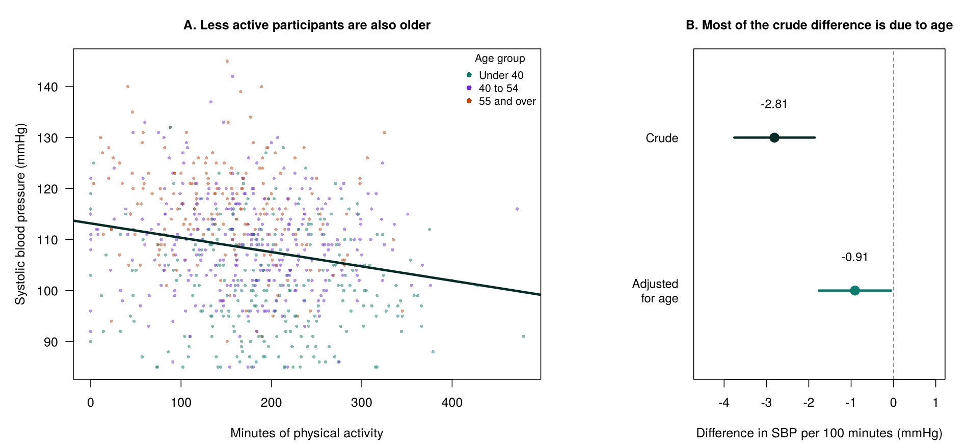
Among the 768 participants with blood pressure, age and physical activity recorded, each additional 100 minutes of activity is associated with a systolic blood pressure 2.81 mmHg lower (95% CI 1.86 to 3.76 mmHg lower). Activity and age are negatively correlated (r = −0.27), and blood pressure rises by about 0.43 mmHg per year of age. When age is added to the model, the difference per 100 minutes falls to 0.91 mmHg (95% CI 0.06 to 1.76 mmHg lower, p = 0.037), a reduction of about two thirds. Most of the crude association reflects the fact that the more active participants are younger.
Explaining a change like this means describing both links of the confounder: age is related to the exposure, because the more active participants are younger, and to the outcome, because blood pressure rises with age. The crude estimate was therefore exaggerated. Both models use the same 768 people, so the change reflects the adjustment for age alone, and question 3 of Activity 3.1 prints the share of the crude coefficient that disappears. Age cannot lie on the path from activity to blood pressure, because activity cannot change a person’s age, so age is a confounder rather than an intervening variable. A smaller adjusted difference is also not the same as no difference: 0.91 mmHg per 100 minutes remains after adjustment.
A two-variable test cannot hold age constant while comparing levels of activity. Regression can, and the next subsection introduces it with a single predictor.
Linear regression describes how the average of a continuous outcome changes with one or more predictors. With one predictor, it fits a straight line, which Equation 3.1 writes as a model for the outcome of each person.
The fitted line for age is SBP = 87.9 + 0.45 × age. The intercept, 87.9 mmHg, is the predicted value at age 0, which is outside the data and has no practical meaning here; it fixes the height of the line. The slope, 0.45 mmHg per year, is the quantity of interest, because it says that each additional year of age goes with a predicted systolic blood pressure about 0.45 mmHg higher.
No straight line passes through every point, so each person sits some distance above or below the line. The residual for each person is the observed blood pressure minus the value on the line. By this we mean the part of a person’s blood pressure that the line does not account for. Many different lines could be drawn through the same cloud of points, and a rule is needed to choose one. Ordinary least squares (OLS) is that rule: it chooses the intercept and slope that make the sum of the squared residuals as small as possible. The residuals are squared for two reasons. First, squaring makes every residual positive, so points above and below the line cannot cancel each other out. Second, squaring gives large misses much more weight than small ones, so the chosen line is pulled strongly towards any point that would otherwise lie far from it. This is also why, as Interactive 3.1 shows, one extreme point can pull the line towards itself.
R stores the fitted value and the residual of every person, in fitted(model) and residuals(model). Because a residual is the observed value minus the fitted value, a positive residual means that the person lies above the line and a negative residual that the person lies below it. Real people scatter around the line, so least squares does not make any single residual zero; it makes the sum of the squared residuals over all people as small as possible.
Click each of the three cards below to review the intercept, the regression coefficient and the error term of Equation 3.1, including the assumptions about the errors that Section 2 checks.
The intercept and the slope fix the line, and the error term recognises that people scatter around it.
Interactive 3.1 shows least squares at work. Click on the chart to add points and watch the line, the residuals and R² update; then load a random sample and press “Add an outlier” several times to see how one unusual point can pull the line.
Click anywhere on the chart to add a point. Click on an existing point to remove it. The least-squares line, residuals, R², and standard error of the slope update live. Hovering over, or tapping, any label below the chart shows a plain-language definition of that number. Add an extreme outlier and watch one observation pull the line (Cook, 1977; Belsley, Kuh, & Welsch, 1980).
A point far from the average value of the predictor tilts the line much more than a point near the middle, an idea that returns in the diagnostic checks of Section 2. The next subsection shows that this simple line already reproduces the familiar tests, and then adds further predictors.
The four tests in Table 3.1 each have a regression counterpart, listed in Table 3.2, so regression provides one framework for all of them. Figure 3.2 illustrates this for blood pressure by smoking status.
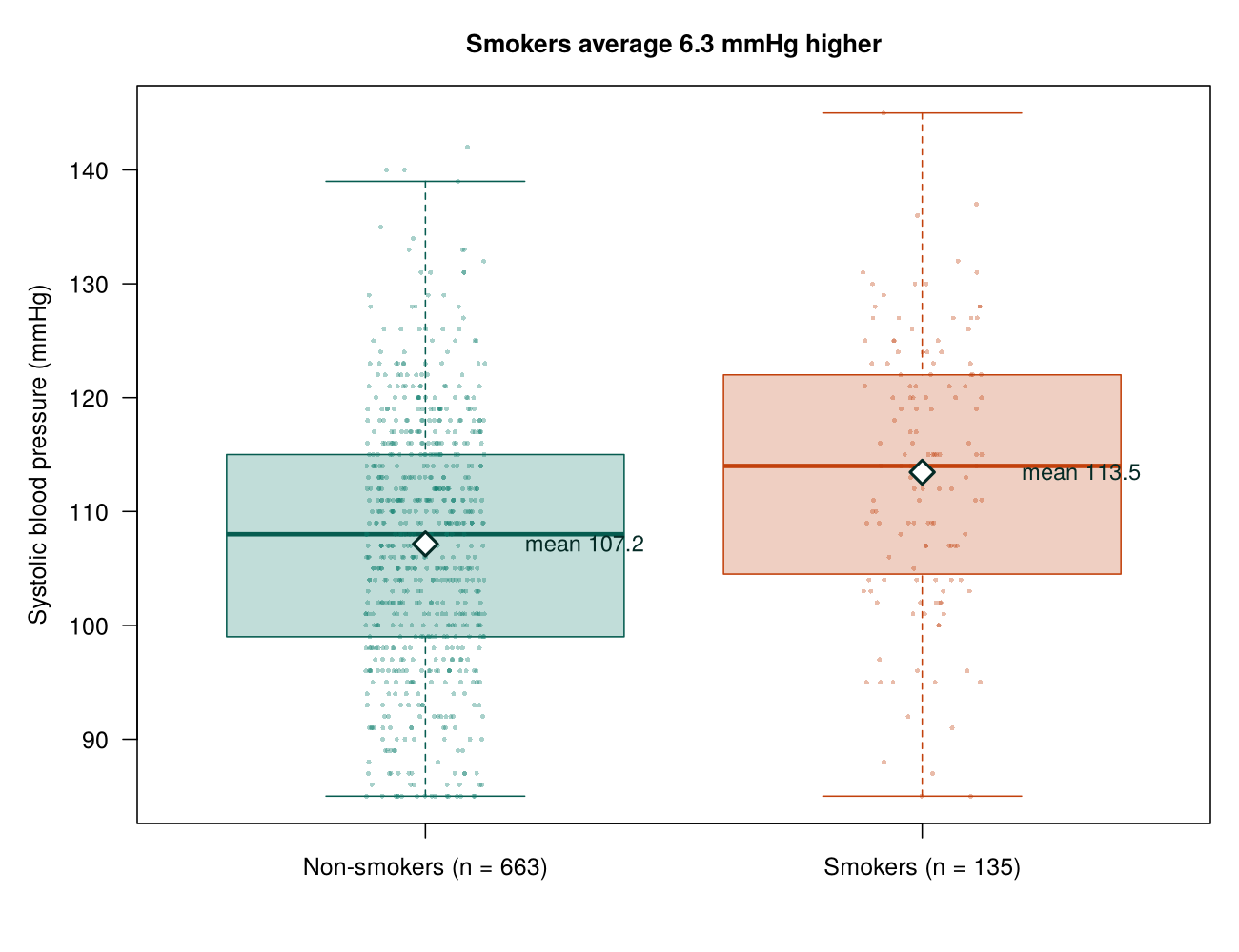
A regression with a single binary predictor reproduces the t-test. In lm(systolic_bp ~ smoker), the intercept (107.16 mmHg) is the mean for non-smokers, the reference group, and the slope for smokerYes (6.30 mmHg) is the difference between the two means. Its t statistic (6.01) and p-value (2.9 × 10⁻⁹) match those of t.test(..., var.equal = TRUE) exactly. A regression with a categorical predictor of three or more groups reproduces the one-way ANOVA, and the F-test printed at the bottom of its summary() is the ANOVA F-test. With one numeric predictor, the slope equals the correlation multiplied by the ratio of the standard deviations of the outcome and the predictor, and the R² of the regression equals the squared correlation, 0.29 for age.
With one predictor, regression reproduces the familiar tests. Adding further predictors is how regression takes confounders such as age into account.
A multivariable regression includes several predictors. Each coefficient then describes the change in the average outcome for a one-unit change in its predictor among people with the same values of the other predictors. By this we mean that the model compares like with like: it estimates how the outcome differs between people who differ in one predictor but are alike in all the others that the model contains. For example, in the physical activity example, the coefficient of −0.0091 mmHg per minute in the model with age compares people of the same age. Because age is held fixed in this comparison, the younger age of the more active participants can no longer make activity look more protective than it is. This property, adjustment for the other variables in the model, is the main reason regression is used in epidemiology, where randomisation is usually not possible and confounders must be dealt with in the analysis instead.
A multivariable coefficient is a difference in averages between such people, not a fixed change in every person. It is also adjusted only for the variables in the model: a confounder that was never measured, or was left out, can still bias it. Expand the three panels below for more on why multivariable models are used, how a confounder differs from an intervening variable, and the trade-offs in choosing which variables to include.
In observational studies, incorporating more than one predictor almost always leads to a more complete understanding of how the outcome varies, and it decreases the chance that the regression coefficients for exposures of interest are biased by confounding variables. A confounding variable that is included in the equation is adjusted for and therefore cannot bias the βs. A confounding variable that is omitted from the equation can still bias them, that is, push them systematically away from the true values, which is why the choice of variables to include matters.
Intervening variables, also called mediators, lie on the causal path between the exposure and the outcome. By this we mean that the exposure changes the intervening variable, and the intervening variable in turn changes the outcome, so it carries part of the effect of the exposure. For example, weight gain may lie on the path from physical inactivity to high blood pressure: inactivity leads to weight gain, and weight gain raises blood pressure. A confounder is different, because it is a common cause of the exposure and the outcome rather than a step between them. Provided the model contains no intervening variables and no variables that are themselves effects of the outcome, no variable in the regression equation confounds the βs. If intervening variables are included, however, the coefficient for the exposure no longer estimates its total causal effect. This is because part of that effect travels through the intervening variable, and holding the intervening variable constant removes that part. In the example, adjusting for weight would compare inactive and active people of the same weight, and so would remove the share of the effect of inactivity that works by raising weight. The possibility that an important confounder was never measured, and was therefore omitted from the model, can never be ruled out completely.
A major trade-off in model building is to include the necessary confounding variables while leaving out variables of little importance. Including too many unimportant variables increases the number of βs estimated and may lead to poor performance of the equation on future datasets. Also, having to measure unnecessary variables increases the cost of future work.
The second panel matters most for later sections: adjustment removes confounding only by variables that were measured and included, and adjusting for an intervening variable changes what the coefficient estimates. Section 4 returns to both points when it chooses variables from a causal diagram.
A multivariable model has one outcome and several predictors. A multivariate model has several outcomes analysed together. The models in this course are multivariable.
Activity 3.1 practises everything in this section. Run along to carry out the four tests in Table 3.1 on the PHAA survey, show that a regression with one binary predictor reproduces the t-test, and add age to the physical activity model, answering three questions in the style of the midterm along the way.
Text version of the activity: the code of the run-along script, its console output and notes on reading it.
phaa <- read.csv("https://heal-learn.ca/r-activities/data/phaa_survey_clean.csv")   # course data, read from the website
phaa$smoker <- factor(phaa$smoker, levels = c("No", "Yes")) # "No" = referencecor.test(phaa$age, phaa$systolic_bp) # two numeric variables
t.test(systolic_bp ~ smoker, data = phaa, var.equal = TRUE) # two group means
round(tapply(phaa$systolic_bp, phaa$region, mean, na.rm = TRUE), 1)
summary(aov(systolic_bp ~ region, data = phaa)) # three or more means
phaa$elevated_bp <- factor(ifelse(phaa$systolic_bp >= 120, "Yes", "No"),
levels = c("No", "Yes")) # 120 mmHg or more
tab <- table(phaa$smoker, phaa$elevated_bp)
tab # counts
round(prop.table(tab, margin = 1), 3) # share with elevated BP
chisq.test(tab) # two categorical variablesReading the output. The correlation is 0.54 (95% CI 0.49 to 0.59) for the 796 people with both measurements (df = 794 is n − 2). t.test() subtracts the second group from the first, so its interval, printed as −8.35 to −4.24, means that smokers average between 4.24 and 8.35 mmHg more than non-smokers; the regression in part 3 prints the difference itself, 6.30 mmHg. The Pr(>F) column gives the ANOVA p-value of 0.139. The rows of prop.table() give the share with elevated blood pressure in each smoking group, and R applies Yates' continuity correction to a two-by-two table by default.
fit_smk <- lm(systolic_bp ~ smoker, data = phaa)
summary(fit_smk)$coefficientsThe intercept is the mean for non-smokers (107.16 mmHg), the reference group, and the smokerYes slope is the difference between smokers and non-smokers (6.30 mmHg), with the same t value and p-value as the t-test above (the sign of t is reversed).
act <- na.omit(phaa[, c("systolic_bp", "phys_act_min", "age")])
nrow(act)                                 # the same people in both models
crude <- lm(systolic_bp ~ phys_act_min, data = act)
adjusted <- lm(systolic_bp ~ phys_act_min + age, data = act)
round(summary(crude)$coefficients, 4)
round(summary(adjusted)$coefficients, 4)
100 * coef(crude)[["phys_act_min"]]       # per 100 minutes, crude
100 * coef(adjusted)[["phys_act_min"]] # per 100 minutes, adjustedBoth models use the same 768 people, so the change in the coefficient for physical activity, from −2.81 to −0.91 mmHg per 100 minutes, reflects the adjustment for age alone. The second line of your own code for question 3 prints the share of the crude coefficient that disappears when age is added.
Answer each question from your own output, as on the midterm: name the test, give each number its units and its comparison, and judge the confounder.
1. For each of the four comparisons on lines 11 to 20, name the test and explain why it fits the types of the two variables, as you would when choosing the statistic and test for each row of a Table 1. Interpret the difference between smokers and non-smokers in plain words, with its 95% confidence interval and p-value, and state what the region and chi-square results show.
2. Using the output of lines 24 and 32 (fit_smk and adjusted), interpret the intercept and the coefficients of each model, attaching units to each and naming the comparison each coefficient makes. What does fit_smk show about the t-test?
fit_smk, the intercept (107.16 mmHg) is the mean systolic blood pressure of non-smokers, the reference group. The smokerYes coefficient (6.30 mmHg) means that smokers have a mean systolic blood pressure 6.30 mmHg higher than non-smokers; its t value (6.01) and p-value are the same as those of the t-test, so a regression with one binary predictor is the t-test written as a model. In adjusted, the intercept (90.47 mmHg) is the predicted systolic blood pressure for a person aged 0 who reports no physical activity, which lies outside the data, so it only fixes the height of the line. Each additional minute of physical activity is associated with a mean systolic blood pressure 0.0091 mmHg lower (0.91 mmHg lower per 100 minutes), holding age constant (p = 0.037). Each additional year of age is associated with a mean systolic blood pressure 0.43 mmHg higher, holding physical activity constant (p < 0.001).3. Run your own code: at the end of the script, type cor.test(act$age, act$phys_act_min) and round(1 - coef(adjusted)[["phys_act_min"]] / coef(crude)[["phys_act_min"]], 2) on two lines and run them. The second line prints the share of the crude coefficient for physical activity that disappears when age is added. Is age a confounder of the association between physical activity and systolic blood pressure? Name its role and the evidence for each of its links, state the consequence of leaving age out of the model, and say how much of the crude association it accounts for.
The output of the activity reproduces the estimates quoted in 1.2, 1.3 and 2.2, including the change in the coefficient for physical activity when age is added. This section has shown how to choose and read a two-variable test, how confounding can distort it, and how regression reproduces the simple tests and adjusts each coefficient for the other predictors. The knowledge check that follows reviews these points.
cor.test()); a numeric outcome compared across two groups calls for a t-test (t.test()), and across three or more groups a one-way ANOVA (aov()); and two categorical variables call for a chi-square test (chisq.test()). Each test has a backup for when its assumptions look doubtful: a rank-based test (Spearman's ρ, Mann-Whitney, Wilcoxon signed-rank for paired data, or Kruskal-Wallis) when the outcome is skewed or ordinal, and Fisher's exact test when an expected count in a 2 × 2 table falls below about 5. A common trap is to choose the test from how a variable is stored rather than what it means: a rating stored as the numbers 1 to 5 is still ordinal, and a variable coded 0 and 1 is still categorical. Before you name a test, also check whether the groups are independent or paired, and for a chi-square test read the expected counts from R: chisq.test(tab)$expected prints them (each is row total × column total ÷ grand total), and R warns that the chi-square approximation may be incorrect when any of them is below 5.t.test(systolic_bp ~ smoker, data = phaa, var.equal = TRUE) subtracts the second group from the first, so it prints the interval as −8.35 to −4.24, which you would report as smokers being 4.2 to 8.4 mmHg higher.(crude - adjusted) / crude gives 0.68), and make sure both models used the same people, so that the change reflects the adjustment alone.fitted(model) and residuals(model). With the PHAA line SBP = 87.9 + 0.45 × age, a 60-year-old lies on the line at about 115 mmHg, so a reading of 120 mmHg has a residual of about +5 mmHg, a point above the line. Two traps to avoid are reading the sign the wrong way round (a residual is always observed minus fitted, so a positive residual lies above the line and a negative one below it) and over-reading the intercept, which here describes a person aged 0, outside the data, and only fixes the height of the line.lm(systolic_bp ~ smoker) gives an intercept equal to the non-smokers' mean (107.16 mmHg) and a slope equal to the difference in means (6.30 mmHg), with the same t value and p-value as the classic t-test. Whenever you interpret a multivariable coefficient, name what is held constant, and remember the limit: a model adjusts only for the confounders that were measured and included, so an unmeasured confounder can still bias the estimate.1. A health unit asks adults in three neighbourhoods to rate their stress on a five-point scale, from 1 (none) to 5 (extreme), and wants to know whether the ratings differ between the neighbourhoods. Which test is most suitable?
2. A two-sample t-test compares HbA1c (%) between adults with and without a family history of diabetes. Those with a family history average 0.40 percentage points higher (95% CI 0.10 to 0.70, p = 0.01). Which interpretation is correct?
3. In a workplace survey, employees who walk to work have a mean systolic blood pressure 4.0 mmHg lower than employees who drive. The walkers are also younger on average, and blood pressure rises with age. When age is added to the regression, the difference falls to 1.2 mmHg. Which conclusion is best supported?
4. A simple linear regression of systolic blood pressure (mmHg) on age (years), saved as fit, gives the line SBP = 90 + 0.5 × age. Person 12 in the data is 40 years old and has an observed systolic blood pressure of 115 mmHg, and R prints the values below for this person. What does the residual mean?
5. A linear model for systolic blood pressure (mmHg) is fitted with lm(sbp ~ salt_g + age), where salt_g is daily salt intake in grams. The coefficient for salt_g is 1.5. Which statement interprets it correctly?
6. A health unit measured lung function as FEV1 (litres) in 460 adults. A two-sample t-test shows that adults who live within 200 m of a highway have a mean FEV1 0.22 L lower than adults who live further away (95% CI 0.12 to 0.32 L, p < 0.001). Smoking is more common near the highway (35% of residents against 15%), so a regression that adds smoking was also fitted, with the output below. Which statement interprets near_hwyYes correctly?
near_hwyYes row (−0.140 L, p = 0.005), the other predictor in the model (smoking) and the crude difference from the t-test (0.22 L). In a multivariable model each coefficient compares people who differ in that predictor but have the same values of the other predictors, here the same smoking status. Smoking is related to the exposure (35% of residents near the highway smoke, against 15% further away) and to the outcome (smokers have a mean FEV1 0.40 L lower), which makes it a confounder of the crude comparison, so part of the 0.22 L difference reflected smoking rather than the highway. Option c is the tempting error: a smaller adjusted difference is not the same as no difference, and 0.14 L remains after adjustment (p = 0.005). Option b describes a fixed effect in every person rather than a difference in averages, and option d ignores the adjustment for smoking. (Section 1, 1.3 How Confounding Distorts a Two-Variable Comparison and 2.2.2 Adjusting for the Other Predictors; Objectives 1.3 and 2.2)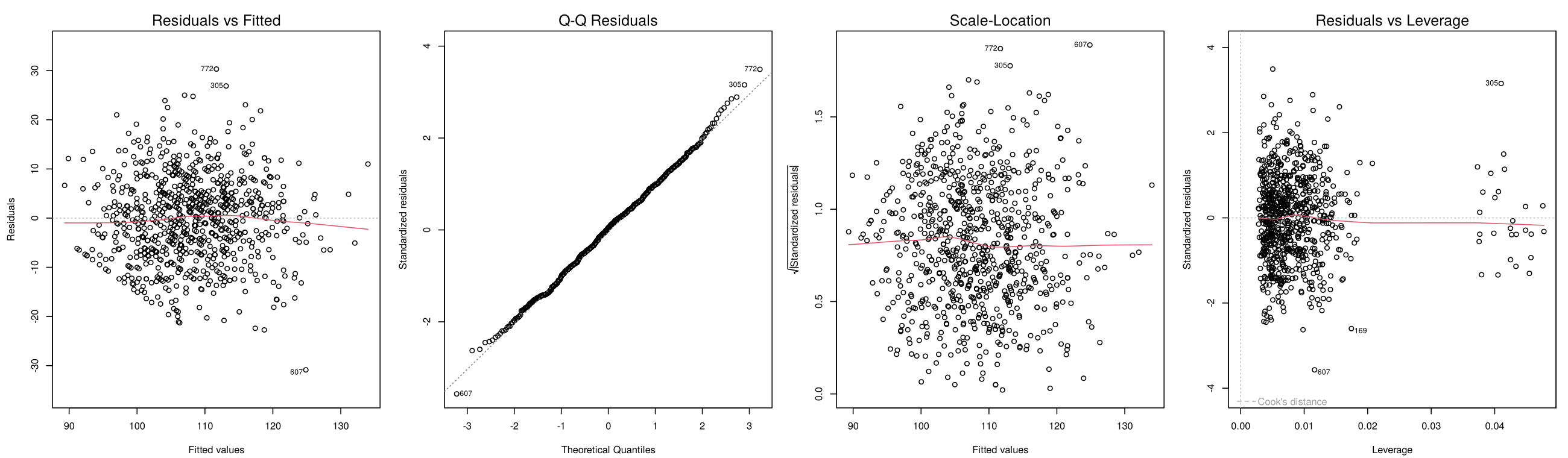
This section fits a multivariable linear regression for systolic blood pressure and asks whether the model can be trusted. It explains how to read each coefficient, including those for categorical, centred and log-transformed predictors; how to test each coefficient and judge the fit of the whole model; how to check the LINE assumptions with the four diagnostic plots and formal tests; how to find influential observations and collinear predictors; and what to do when a check fails. The model has five predictors (age, gender, smoking, BMI and the depression score) and uses the 795 PHAA participants with complete data for these variables.
lm() and interpret its intercept and coefficients, stating the units, the comparison each makes (per unit of the predictor or against the reference category) and what is held constant, including centred and log-transformed predictors.The model is written in R as lm(systolic_bp ~ age + gender + smoker + bmi + dep_score, data = cc), where cc holds the complete cases. Table 3.3 gives each coefficient with its 95% confidence interval and an interpretation. Every estimate is adjusted for the other predictors in the model.
Table 3.3. Estimates, 95% confidence intervals and interpretations for the five-predictor linear regression of systolic blood pressure.
| Predictor | Estimate (mmHg) | 95% CI | Interpretation |
|---|---|---|---|
| Intercept | 71.14 | 66.59 to 75.69 | The predicted value for a non-smoking man aged 0 with a BMI and depression score of 0, which is outside the data and has no practical meaning. |
| Age | 0.43 | 0.38 to 0.47 | Each additional year of age is associated with a systolic BP 0.43 mmHg higher (4.3 mmHg per decade). |
| Woman vs man | −0.34 | −1.58 to 0.90 | Women average 0.34 mmHg lower than men; the interval includes 0. |
| Non-binary vs man | −0.61 | −4.03 to 2.81 | The wide interval reflects the small group of 27 non-binary participants. |
| Smoker vs non-smoker | 6.15 | 4.49 to 7.80 | Smokers average 6.15 mmHg higher than non-smokers with the same age, gender, BMI and depression score. |
| BMI | 0.43 | 0.23 to 0.63 | Each additional unit of BMI is associated with a systolic BP 0.43 mmHg higher. |
| Depression score | 0.38 | 0.30 to 0.46 | Each additional point on the depression score is associated with a systolic BP 0.38 mmHg higher. |
The smoking estimate in this model (6.15 mmHg) is close to the unadjusted difference of 6.30 mmHg from Section 1, but Section 4 shows that this similarity hides two changes in opposite directions: adjustment for the confounders lowers the estimate, and adjustment for BMI, a mediator, raises it.
Every interpretation in Table 3.3 follows the same pattern, which is worth committing to memory.
Every interpretation of a linear regression coefficient names four things: the size of the coefficient in the units of the outcome, the comparison it makes, what is held constant, and the uncertainty. For example: "Each additional year of age is associated with a mean systolic blood pressure 0.43 mmHg higher (95% CI 0.38 to 0.47), holding gender, smoking, BMI and depression score constant."
Two kinds of predictor need extra care: categorical predictors, whose coefficients depend on the reference category, and predictors whose zero lies outside the data, which make the intercept hard to read.
A regression needs numbers, so a categorical predictor such as gender cannot enter the model as words. Instead, a categorical predictor with k categories enters the model as k − 1 indicator variables, each coded 1 for one category and 0 otherwise. By this we mean that gender, with three categories, becomes two yes-or-no columns: one that equals 1 for women and 0 for everyone else, and one that equals 1 for non-binary participants and 0 for everyone else. A man has 0 in both columns, so no separate column is needed for men. The category without an indicator is the reference category, chosen in R with factor(..., levels = ) or relevel(). Because the reference category is the baseline that every indicator is measured against, each coefficient is the difference in the mean outcome between its category and the reference category. For example, genderWoman (−0.34 mmHg) compares women with men, not with everyone else. Changing the reference category changes the numbers printed, because each coefficient then answers a different comparison, but it does not change the model or its predictions.
The intercept is the predicted mean outcome when every predictor equals 0 and every categorical predictor is at its reference category. In Table 3.3 that describes a non-smoking man aged 0 with a BMI and depression score of 0, so it has no practical meaning. Centring a predictor, that is, subtracting a meaningful value from it, moves its zero into the data without changing its slope. By this we mean that the predictor is measured as a distance from a chosen value rather than from zero, so a value of 0 on the new scale now describes a real and typical person. The slope does not change, because a one-unit step is the same step on either scale; only the starting point of the line, and so the intercept, is redefined. With age entered as age − 50, the slope for age stays at 0.43 mmHg per year, and the intercept becomes 92.5 mmHg, the prediction for a 50-year-old (still at a BMI and depression score of 0, so those would be centred too for a fully meaningful intercept). A rating recoded from 1 to 5 into −2 to 2 is centred in the same way: its zero is the middle category, so the intercept describes a person in that category.
A right-skewed predictor that includes zeros, such as minutes of activity or hours of volunteering, is often entered as ln(x + 1). A right-skewed predictor is one in which most people have small values and a few have very large ones, and those few large values can dominate the fitted line. Taking the natural log pulls the long right tail in, so that the step from 10 to 100 minutes counts about as much as the step from 100 to 1000 minutes. The 1 is added because the log of 0 is undefined, and adding 1 keeps the people who report no activity in the model. The cost of the transformation is a less direct interpretation. Its coefficient is the change in the mean outcome for each one-unit increase in ln(x + 1), and a one-unit increase on that scale means multiplying (x + 1) by e, about 2.72. In other words, the coefficient now describes the effect of a proportional increase in the predictor rather than an increase of a fixed number of minutes. The predicted difference between two values x1 and x2 is β × [ln(x2 + 1) − ln(x1 + 1)]. In the PHAA survey, lm(systolic_bp ~ log(phys_act_min + 1) + age) gives a coefficient of −0.66 mmHg (p = 0.10). R gives the predicted difference between 50 and 150 minutes of activity in one line, coef(fit)["log(phys_act_min + 1)"] * (log(151) - log(51)), which prints −0.72: moving from 50 to 150 minutes predicts a blood pressure 0.72 mmHg lower, holding age constant. An interpretation "per unit of ln(minutes + 1)" is correct; translating it into the original units makes it easier to read.
Each estimate in Table 3.3 comes with a standard error, and the next subsection explains how it is used to test the coefficient and to build its confidence interval.
Each row of the summary() output gives a t-test of whether that coefficient differs from zero. A coefficient of zero would mean that the predictor has no association with the outcome once the other predictors are held constant, so this is the natural value to test against. The test needs the standard error of the coefficient, which is the typical amount by which the estimate would vary if the study were repeated on new samples of the same size. Because a raw estimate of 6 mmHg could be large or small depending on how precisely it is measured, the test scales the estimate by its standard error. The t value is the estimate divided by its standard error, so it says how many standard errors the estimate lies from zero. For example, the t value of 7.28 that R prints for smoking says that the smoking estimate lies about seven standard errors from zero, which would be very unusual if the true coefficient were 0. The p-value in the Pr(>|t|) column is the probability of an estimate at least that far from zero if the true coefficient were 0; it is not the probability that the coefficient is 0. The 95% confidence interval, from confint(), is approximately the estimate plus or minus 1.96 standard errors, and it shows both the size of the effect and how precisely it is estimated. For smoking, confint() prints 4.49 to 7.80 mmHg, the range of adjusted differences that are consistent with the data.
The interval and the test agree: a 95% interval that excludes 0 goes with p < 0.05, and one that includes 0 goes with p ≥ 0.05. An interval that includes 0, such as −1.58 to 0.90 mmHg for women against men, means that the data are compatible with no difference, but it does not prove that there is none, so it is reported as no clear evidence of a difference. A coefficient also describes a difference in averages, not a fixed change in every person. The interval is often more useful than the p-value, because a p-value on its own says nothing about how large an effect is.
The confidence interval for a coefficient describes uncertainty about where the line lies. Expand the panel below to see how that uncertainty combines with the scatter of individual people when the model is used to predict.
Two sources of uncertainty stack when you use a fitted model to predict. The first is uncertainty about where the regression line itself sits, captured by the standard error of the fitted value. By this we mean that a different sample would have given a slightly different line, so the average blood pressure that the line predicts for, say, 50-year-olds is itself only an estimate. The second is the natural scatter of an individual observation around that line. Even if the line were known exactly, two 50-year-olds would not have the same blood pressure, because individuals differ from the average for their age. A confidence interval for the mean of Y at a chosen value x* (a particular value of the predictor, such as an age of 50) uses only the first source: Ŷ ± t0.025·SE, where t0.025 is the critical t value that leaves 2.5% of the t distribution in each tail (about 1.96 in large samples). A prediction interval for a single new individual adds the second source, so it is always wider than the confidence interval. Both intervals widen as x* moves further from the mean of X1, because the line is pinned down most tightly near the centre of the data.
A prediction for one new person is therefore always less certain than the estimate of the average at the same predictor value.
p-values themselves vary from one study to the next. Interactive 3.2 runs many imaginary studies with a chosen true effect and sample size. Run a few hundred studies with no true effect, then switch to a real effect and run them again, and watch how the p-values are spread: evenly between 0 and 1 when there is no effect, and piled up near zero when there is one, more so as the sample grows.
Run hundreds of simulated studies. Each study fits a regression of Y on X with a chosen true effect and sample size. Watch the distribution of p-values build up. With no real effect, p-values are uniform on [0,1], meaning that every value between 0 and 1 is equally likely. With a real effect, p-values pile up near zero. Power, the chance that a study detects an effect that is really present, equals the proportion of p-values below α, the significance threshold (usually 0.05).
A scatter of n points; black line = OLS fit; t-statistic and p-value displayed.
Histogram of all p-values run so far. Red region = p < α (significant).
The simulator shows that a single p-value is an unreliable summary on its own, which is why the estimate and its confidence interval are always reported with it. The next subsection turns from single coefficients to the model as a whole.
The last three lines of the summary() output describe the whole model rather than any single coefficient. R² is the share of the variation in the outcome that the predictors explain (0.414). By this we mean that people’s systolic blood pressures differ from the overall mean, and the model accounts for about 41% of those differences through age, gender, smoking, BMI and depression score; the remaining 59% is left in the residuals. R² has a weakness, however. Because R² always rises when a predictor is added, even a useless one, a model can look better simply by containing more variables. For this reason the adjusted R² applies a penalty for each predictor (0.409). It rises only when a new predictor explains more variation than a predictor unrelated to the outcome would typically explain by chance, so it is the statistic to give when a question asks for the variance explained after penalising the model for unnecessary predictors, or when models of different sizes are compared.
The residual standard error (8.70 mmHg) describes fit in a different way. It is the typical distance between an observed value and the model’s prediction, in the units of the outcome, so it is not a share of the variance. For example, it says that the model’s predicted blood pressure for a person is typically off by roughly 9 mmHg, which is a useful reminder of how much individuals vary around the average for people like them. Finally, the F-test asks whether the predictors together explain more variation than chance. Its null hypothesis is that every coefficient other than the intercept is zero, so a small p-value means that at least one predictor is associated with the outcome (F = 92.7 on 6 and 788 degrees of freedom, p < 0.001). A low R² is common in health research and does not by itself mean that a model is wrong. This is because health outcomes depend on many factors that a survey does not measure, so a model can estimate an association accurately while still leaving most of the variation between people unexplained.
Expand the three panels below for the formulas behind R² and adjusted R², the partial F-test for a group of predictors, and the reasons why the overall F-test is hard to interpret in observational data.
R² (the coefficient of determination) describes the amount of variance in the outcome “explained” by the predictor variables. One formula: R² = SSM/SST = 1 − (SSE/SST). By this we mean that the total variation in the outcome around its mean (SST) is split into the part the model accounts for (SSM) and the part left in the residuals (SSE), and R² is the first part as a share of the total. Unfortunately, R² always increases as variables are added to the model, because even a predictor unrelated to the outcome will, by chance, account for a little of the variation in a particular sample. The adjusted R² = 1 − (MSE/MST) addresses this. It replaces each sum of squares with a mean square, that is, a sum of squares divided by its degrees of freedom, so every added predictor uses up a degree of freedom and must explain enough variation to pay for it. As a result, the adjusted R² adjusts for the number of predictors and is useful for comparing models with different numbers of variables.
Sometimes it is necessary to simultaneously evaluate the significance of a group of X-variables (e.g., a set of indicator variables for a nominal variable). For example, gender enters the blood pressure model as two indicators, and the question of interest is whether gender as a whole matters, not whether women differ from men or non-binary participants differ from men taken one at a time. To answer it, two models are fitted: the full model, which contains the group, and the reduced model, which is identical except that the group is left out. The SSE of the full model is compared with the SSE of the reduced model using a partial F-test. Because the reduced model has fewer predictors, its SSE is always at least as large; the test asks whether the reduction in SSE gained by adding the group is larger than chance alone would produce. In this way it shows whether the set of variables as a group contributes significantly to the model.
The F-test has a straightforward interpretation only in a controlled experiment, where the investigators set the values of the X-variables themselves, for example by assigning treatments. In observational studies, where the X-variables are measured as they occur, the F-statistic also depends on how many candidate variables were available, how strongly they are correlated with one another, the total number of subjects, and the method used to choose which variables to keep (variable selection). Most variable selection methods keep the combination of variables that makes F largest, so the observed F overstates the significance that the model would show in a new sample.
The partial F-test in the second panel returns in Section 4, where it compares nested models. Worked Example 3.2 opens the analysis of variance table for the blood pressure model to show where R², adjusted R² and the residual standard error come from; watch how the residual row and the sums of squares connect to the numbers that summary() prints.
anova(model) prints the sequential analysis of variance table for the five-predictor model. Each row gives a term's degrees of freedom (Df), its sum of squares (Sum Sq), its mean square (Mean Sq = Sum Sq ÷ Df) and its F value (the term's Mean Sq divided by the residual Mean Sq). A categorical predictor with k categories uses k − 1 degrees of freedom, so gender, with three categories, uses 2. The table is sequential: each row shows what that term adds after the terms listed above it.
Step 1, the residual row. The residual sum of squares (SSE) is 59,585 on 788 degrees of freedom, and the residual Mean Sq, 75.6, is the mean squared error (MSE). Its square root is the residual standard error that summary() prints, 8.696 mmHg. The error degrees of freedom are n − (k + 1), where n is the 795 people and k + 1 counts the six coefficients and the intercept.
Step 2, the total. The Sum Sq column adds up to the total sum of squares (SST), the variation in systolic blood pressure around its mean, on n − 1 degrees of freedom; dividing it by those degrees of freedom gives the total mean square (MST). The model sum of squares (SSM) is the part of SST that the predictors account for, SST − SSE, and SSE is the part they leave unexplained.
Step 3, R² and adjusted R². R² = SSM ÷ SST = 1 − SSE ÷ SST compares sums of squares, and summary(model) prints it as Multiple R-squared: 0.4137, so the predictors explain 41.4% of the variance in systolic blood pressure. Adjusted R² = 1 − MSE ÷ MST compares mean squares instead: because each sum of squares is divided by its degrees of freedom, every added predictor costs a degree of freedom, and the model is penalised for it. R prints this value as Adjusted R-squared: 0.4093, and it is the statistic to use when a question asks for the proportion of variance explained after penalising the model for unnecessary predictors. The values are always read from summary(model); the three steps show what each printed number measures.
The residual row gives the residual standard error, and the comparison of residual and total variation gives R² and adjusted R². All of these statistics, and the tests in 3.1, are trustworthy only when the model’s assumptions hold, which the next subsection checks.
The four main assumptions of linear regression are summarised by the word LINE: Linearity (the average outcome changes in a straight line with each continuous predictor), Independence (one person’s outcome carries no information about another’s), Normality of the residuals, and Equal variance of the residuals at every fitted value. Two further checks, for influential observations and for collinearity, are usually added, and 4.2 describes them. Table 3.4 sets out all six, how each is checked and the result for the blood pressure model.
Table 3.4. The four LINE assumptions and two further checks for linear regression, how each is checked, and the result for the blood pressure model.
| Assumption | What it means | How to check it | Result for this model |
|---|---|---|---|
| Linearity | The average outcome changes in a straight line with each continuous predictor. | Residuals vs Fitted plot; add a squared term and compare models. | Flat smoother; squared age term p = 0.51. |
| Independence | Each observation is unrelated to the others. | Judged from the study design. | One survey row per person. |
| Normality | The residuals are roughly normally distributed. | Q-Q plot; shapiro.test(). | Points on the line; p = 0.62. |
| Equal variance | The residuals have the same spread at every fitted value. | Scale-Location plot; bptest(). | Flat line; p = 0.58. |
| No undue influence | No single observation changes the results much. | Residuals vs Leverage plot; Cook's distance. | Largest Cook's distance 0.061. |
| No strong collinearity | The predictors are not too strongly correlated with each other. | vif(). | All values below 1.12. |
Calling plot() on a fitted lm object in R produces four panels, each of which addresses one or more of the assumptions above. Table 3.5 describes what each panel shows and how a problem appears in it.
Table 3.5. What each of the four diagnostic panels from plot() shows, and how an adequate model and a problem appear in it.
| Panel | What it plots | What an adequate model shows | What a problem looks like |
|---|---|---|---|
| Residuals vs Fitted | Raw residuals against fitted values, with a smoothed trend line | A horizontal band of points centred on zero, with the smoothed line close to flat | A systematic curve indicates a misspecified functional form; a band that widens from left to right indicates non-constant variance |
| Q-Q Residuals | Standardised residuals against the quantiles expected under normality | Points lying close to the diagonal reference line | An S-shaped pattern indicates tails heavier or lighter than normal, meaning more or fewer extreme residuals than a normal distribution would produce; a bend at one end indicates skew; isolated points at either end indicate outliers |
| Scale-Location | The square root of the absolute standardised residuals against fitted values | A flat smoothed line with even vertical scatter | A rising or falling smoothed line, which is the clearest visual signal of non-constant variance |
| Residuals vs Leverage | Standardised residuals against leverage, with dashed contours of Cook’s distance at 0.5 and 1 | All points well inside the contours; in a well-behaved model the contours often fall outside the plotted region altogether | Points beyond a contour, whose removal would move one or more coefficients appreciably |
The panels are read together. A funnel in the first panel that reappears as a rising line in the third is strong evidence of non-constant variance, whereas a single stray point that appears in the second panel and again in the fourth points to influence, and the distributional assumption may still hold for the remaining observations. R labels the three most extreme observations in each panel by row name, which makes it straightforward to inspect those rows directly.
The four panels share a vocabulary. A fitted value is the model's prediction for an observation, and a residual is the observed outcome minus the fitted value. A standardised residual is a residual divided by its estimated standard deviation, so that values beyond about ±2 are unusual and values beyond ±3 are rare. The red line in three of the panels is a smoother that follows the average pattern of the points, and the numbers printed beside a few points are row names, which identify the observations R considers most extreme in that panel.
Figure 3.3 shows the four panels R produces for the blood pressure model in this section, and all four look as an adequate model should. Figures 3.4 to 3.7, in the parts that follow, place a simulated adequate panel beside simulated problem panels so that each pattern can be recognised, and the R code after Figure 3.7 generates the simulated data, so the pictures can be reproduced.
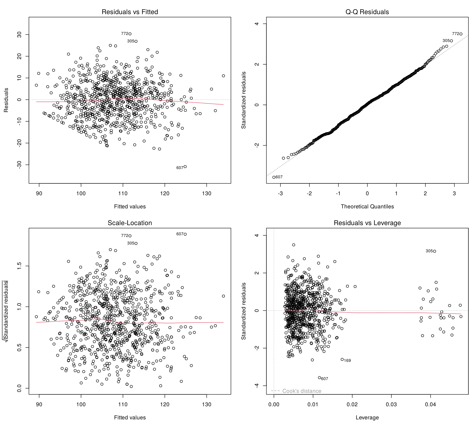
plot(model) for the blood pressure model. Residuals form an even band around zero, the Q-Q points follow the diagonal, the scale-location line is flat, and no point approaches a Cook's distance contour. The vertical cluster at a leverage of about 0.04 is the 27 non-binary participants, whose indicator variable rests on a small group.The Residuals vs Fitted panel plots the raw residuals against the fitted values and shows problems with linearity and with constant variance. Figure 3.4 compares an adequate model with a curved relationship and with errors whose spread grows with the fitted value.
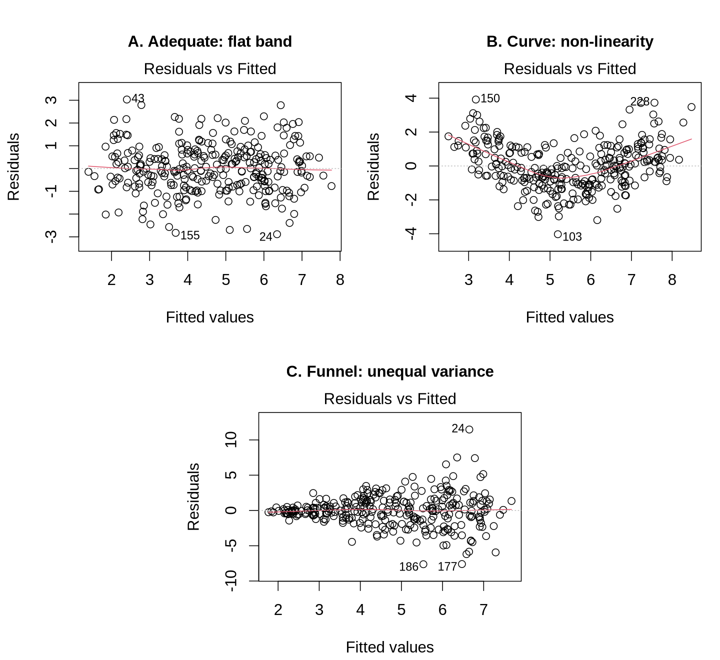
Each point is one observation, placed at its predicted value on the horizontal axis and its residual on the vertical axis. In an adequate model (panel A) the red smoother stays close to the dashed zero line and the vertical spread is similar everywhere. A curved smoother (panel B) means the predictions are systematically too low at both ends and too high in the middle, which is the signature of a non-linear relationship; the response is to model the curve, as 4.3 describes. A band that widens from left to right (panel C) means the errors are larger for some fitted values than for others, which is non-constant variance.
The Q-Q Residuals panel checks whether the residuals are roughly normally distributed. Figure 3.5 compares normal errors with right-skewed and heavy-tailed errors.
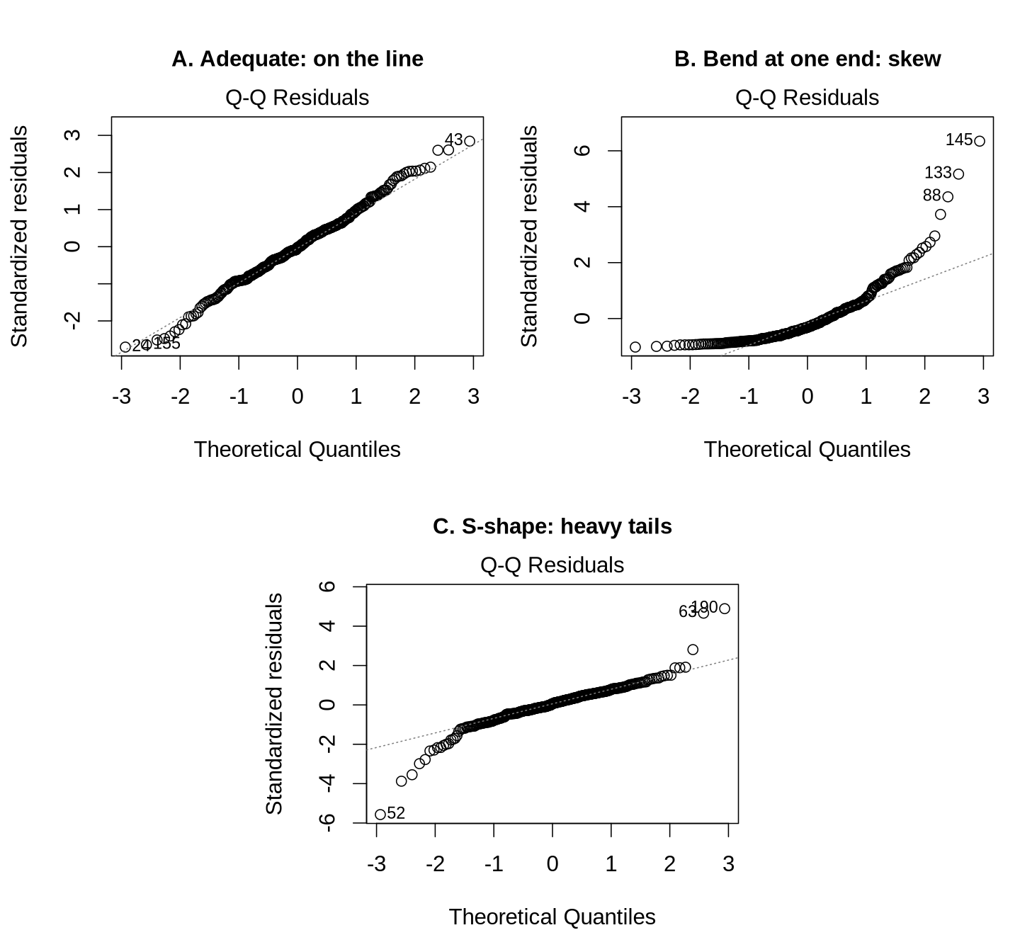
R sorts the standardised residuals from smallest to largest and plots each one against the value expected for its rank if the errors were exactly normal; these expected values are the theoretical quantiles. By this we mean that the smallest residual is paired with the value that the smallest of that many draws from a normal distribution would typically take, the median residual with the middle of the normal distribution, and so on. If the residuals really are normal, each observed value roughly matches its expected value, so normal errors fall along the dashed diagonal. Small wiggles and a few points drifting at the extreme ends occur in any real dataset, as in panel A. A systematic bend at one end (panel B) indicates skewed errors, here a long tail of large positive residuals. An S-shape with both ends pulling away from the line (panel C) indicates heavy tails, meaning more extreme residuals in both directions than a normal distribution would produce.
The Scale-Location panel gives the clearest visual signal of non-constant variance. Figure 3.6 compares constant variance with the funnel-shaped model of Figure 3.4.
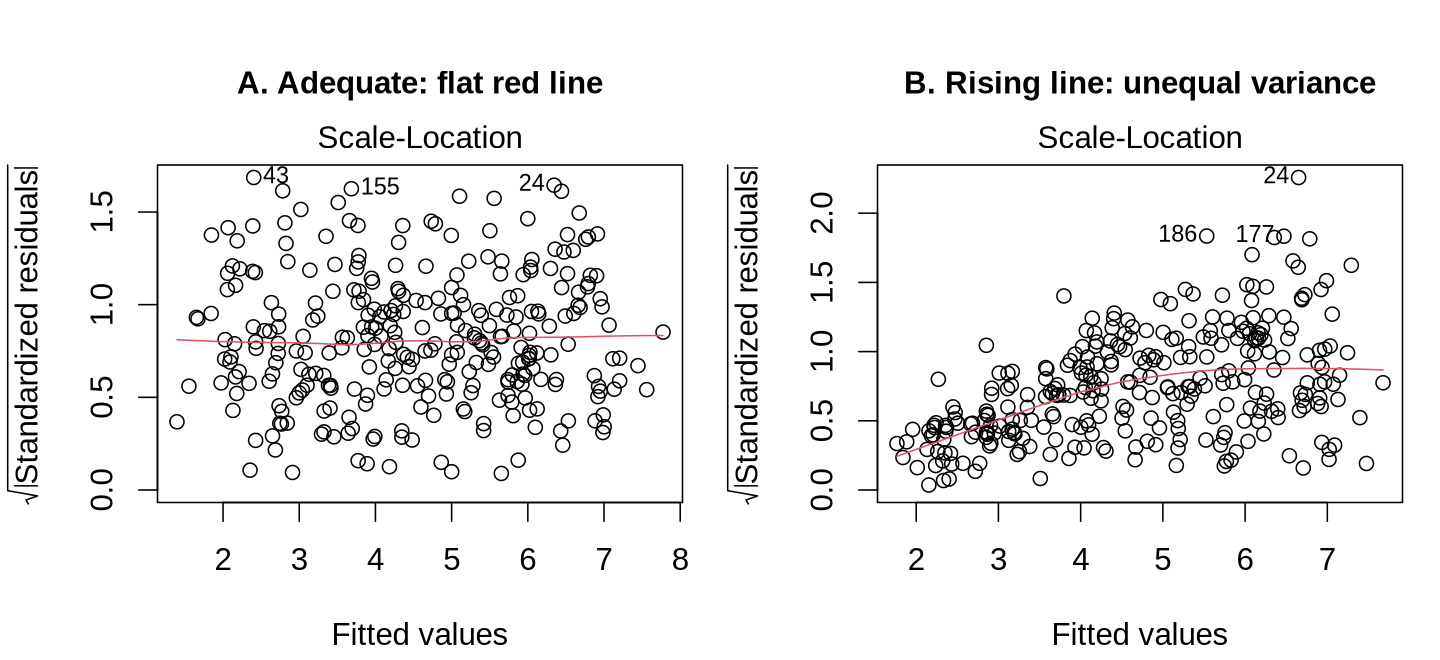
The vertical axis is the square root of the absolute standardised residual, which measures the size of each residual regardless of its sign. A flat red line (panel A) means residuals are of similar size across the range of fitted values. A rising red line (panel B) means residuals grow as the predictions grow, the signature of non-constant variance. This panel often shows the problem more clearly than the Residuals vs Fitted panel, because positive and negative residuals are combined.
The last of the four panels identifies observations with a large influence on the coefficients. Figure 3.7 compares simulated data without an influential point with the same data after one observation is added.
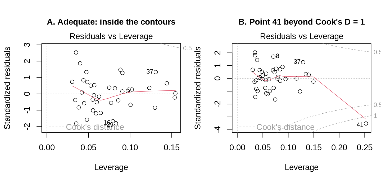
The horizontal axis is leverage, which measures how unusual an observation's combination of predictor values is, and the vertical axis is the standardised residual, which measures how poorly the model predicts it. The dashed grey curves are contours of Cook's distance at 0.5 and 1. Points near the right-hand corners combine high leverage with a large residual and therefore have the greatest influence on the coefficients. In panel A every point lies well inside the contours. In panel B, row 41 has a leverage of 0.25 and a standardised residual of −3.5, which places it beyond the contour of 1 (its Cook's distance is 1.39). Removing that single row moves the slope for x1 from 0.36 to 0.46.
4.2 describes the measures of influence behind this panel. The R code below reproduces the simulated examples in Figures 3.4 to 3.7; run it in RStudio and compare your panels with the figures.
The code below generates every simulated dataset in Figures 3.4 to 3.7. The numbers in plot(model, which = ) select the panel: 1 for Residuals vs Fitted, 2 for Q-Q Residuals, 3 for Scale-Location and 5 for Residuals vs Leverage.
suppressPackageStartupMessages({library(car); library(lmtest); library(sandwich)})
set.seed(410)
n  <- 300
x1 <- runif(n, 0, 10)
x2 <- rnorm(n)
ok     <- data.frame(x1, x2, y = 2 + 0.5 * x1 + 0.3 * x2 + rnorm(n))
curved <- data.frame(x1, x2, y = 2 + 0.5 * x1 + 0.12 * (x1 - 5)^2 + 0.3 * x2 + rnorm(n))
fan    <- data.frame(x1, x2, y = 2 + 0.5 * x1 + 0.3 * x2 + rnorm(n) * (0.2 + 0.35 * x1))
skew   <- data.frame(x1, x2, y = 2 + 0.5 * x1 + 0.3 * x2 + (rexp(n, 1) - 1) * 1.2)
heavy  <- data.frame(x1, x2, y = 2 + 0.5 * x1 + 0.3 * x2 + rt(n, df = 3) * 0.8)
model_ok     <- lm(y ~ x1 + x2, data = ok)
model_curved <- lm(y ~ x1 + x2, data = curved)
model_fan    <- lm(y ~ x1 + x2, data = fan)
model_skew   <- lm(y ~ x1 + x2, data = skew)
model_heavy  <- lm(y ~ x1 + x2, data = heavy)
set.seed(7)
ni  <- 40
xi  <- runif(ni, 0, 10)
xx2 <- rnorm(ni)
e   <- rnorm(ni)
inf <- data.frame(x1 = c(xi, 16), x2 = c(xx2, 0))
inf$y <- c(2 + 0.5 * xi + 0.3 * xx2 + e, 5)
model_inf <- lm(y ~ x1 + x2, data = inf)par(mfrow = c(1, 3))
plot(model_ok, which = 1); plot(model_curved, which = 1); plot(model_fan, which = 1)
plot(model_ok, which = 2); plot(model_skew, which = 2); plot(model_heavy, which = 2)
par(mfrow = c(1, 2))
plot(model_ok, which = 3); plot(model_fan, which = 3)
plot(lm(y ~ x1 + x2, data = inf[1:40, ]), which = 5); plot(model_inf, which = 5)
par(mfrow = c(1, 1))Formal tests can support the plots. For the blood pressure model they all agree with what the panels show: a squared age term does not improve the fit (F = 0.43, p = 0.51), the Breusch-Pagan test finds no evidence of unequal variance (BP = 4.68 on 6 df, p = 0.58), and the Shapiro-Wilk test finds no evidence of non-normal residuals (W = 0.998, p = 0.62). A small p-value from any of these tests signals a problem. Formal tests depend on the sample size, however: in a very large sample they can flag departures too small to matter, and in a small sample they can miss real problems. The plots therefore lead and the tests are reported alongside them, because the test asks whether there is a departure and the plot shows how large it is.
Expand the four panels below for what each test does and where it falls short, and for a plot that finds the predictor behind a curve.
The score test in car::ncvTest(model) asks whether the variance of the errors changes with the fitted values, and the studentised Breusch-Pagan test in lmtest::bptest(model) asks whether it changes with any of the predictors (Breusch & Pagan, 1979). A small p-value from either test indicates non-constant variance. The two tests can disagree, because a variance that depends on one predictor but not on the fitted value is detected by the second test and missed by the first.
shapiro.test(residuals(model)) tests the null hypothesis that the residuals come from a normal distribution (Shapiro & Wilk, 1965). Its power grows with the sample size, so in a sample of several hundred it rejects departures too small to affect the coefficient tests, and in a sample of twenty it can miss departures that matter. The same growth in sample size that makes the test oversensitive also brings the protection of the central limit theorem, under which the sampling distribution of each coefficient approaches normality even when the errors are not normal. The Q-Q plot should therefore govern the judgement, with the formal test reported alongside it.
The Residuals vs Fitted panel shows that the functional form is wrong somewhere without showing where. car::crPlots(model) draws one component-plus-residual plot for each continuous predictor. Each plot takes the part of the prediction that comes from that predictor alone (its coefficient multiplied by its values), adds the residuals back to it, and plots the result against the predictor, which shows the shape of that predictor’s relationship with the outcome after the other predictors are taken into account. A curved smoothed line in one of these plots identifies the predictor whose functional form needs attention, and a squared term or a spline for that predictor is the usual response.
Independence is established mainly by knowing how the data were collected. When the rows have a natural order, such as successive weeks of surveillance data, car::durbinWatsonTest(model) tests for correlation between neighbouring residuals. When observations are clustered, no residual test substitutes for recognising the clustering in the design, and the appropriate response is a model that represents it, such as a mixed model or generalized estimating equations (GEE).
The blood pressure model passed each of these checks. Two further checks, for single observations that drive the results and for predictors that overlap too much, complete the picture.
An influential observation is one that, on its own, changes the results noticeably. By this we mean that the fitted coefficients would be appreciably different if that one person were left out of the data. A point becomes influential when it combines two features: an unusual set of predictor values, which gives it leverage over the line, and an outcome that the model predicts poorly, which gives it a large residual. Cook’s distance, from cooks.distance(model), brings these together. It measures how far the coefficients would move if one observation were removed, and R calculates it for every row. Values above 0.5 warrant investigation and values above 1 are generally treated as serious. A threshold of 4/n is also widely quoted, but it is a liberal screen that flags a few per cent of rows in almost any dataset, so crossing it is a reason to look at a row, not to delete it. In the blood pressure model, 35 people lie above the 4/n line, but the largest Cook’s distance is only 0.061, far below 0.5, so no single person drives the results. Expand the panel below for the three measures that make up influence and the reason why screening thresholds should not be used to delete rows.
Three measures, each with a conventional screening threshold, describe the components of influence. Leverage, from hatvalues(model), flags observations with unusual predictor values, and values above 2p/n, where p is the number of estimated coefficients including the intercept, merit a look. Externally studentised residuals, from rstudent(model), flag outcomes the model predicts poorly, and values beyond about ±3 are unusual, although in a sample of several hundred a handful are expected by chance. Cook’s distance, from cooks.distance(model), combines the two into a single measure of how far the coefficients would move if the observation were removed; values above 0.5 warrant investigation, and values above 1 are generally treated as serious. A threshold of 4/n is also widely quoted, but it is a liberal screen that flags a few per cent of observations in almost any dataset, so it serves to identify rows for inspection. Leverage can arise from a rare category as well as from an extreme numeric value, since every member of a small group has high leverage for that group’s indicator variable. Removing high-leverage rows on the strength of a screen alone can therefore remove an entire small group from the analysis.
That last point applies to this model: the 27 non-binary participants have higher leverage simply because their group is small, and removing them on the strength of a screen would remove a whole group from the analysis.
Collinearity means that predictors are so strongly correlated with one another that their effects are hard to separate. Recall that each coefficient compares people who differ in one predictor but have the same values of the others. When two predictors almost always move together, such as weight and waist circumference, the data contain very few people who are high on one and low on the other, so there is little information with which to make that comparison. The model can still estimate the combined effect of the two, but it struggles to say how much belongs to each.
The variance inflation factor (VIF) measures how serious this problem is for each predictor. The VIF for predictor j is VIFj = 1 ÷ (1 − R²j), where R²j is the R² from regressing that predictor on all the other predictors, so it shows how well a predictor is explained by the others. By this we mean that the VIF asks how much of a predictor’s variation is already carried by the rest of the model. If the other predictors explain none of it, R²j is 0 and the VIF is 1; as they explain more of it, R²j approaches 1 and the VIF grows rapidly. A VIF of 1 means no collinearity, a value above 5 is concerning, and a value above 10 indicates serious collinearity.
Collinearity does not bias a coefficient. It inflates the coefficient’s standard error by about √VIF, which widens the confidence interval and shrinks the t value, so the cost of collinearity is lost precision.
For the blood pressure model, vif(model) gives values below 1.12 for all five predictors, close to the ideal value of 1 and far below the warning thresholds of 5 and 10, so collinearity is not a concern. For a categorical predictor with several indicators, such as gender, vif() reports a generalised VIF (GVIF), which is read like an ordinary VIF. Collinearity between two different predictors, such as two measures of the same thing, is handled by keeping the one with the stronger rationale, combining them into one index, or keeping both and reporting the wider intervals. A predictor and its own square are another common source of serious collinearity, which Worked Example 3.5 shows when a squared age term is added. The blood pressure model passes every check, but many models do not, and the last subsection describes the standard responses.
A failed check calls for a change to the analysis that matches the cause of the problem, rather than deleting data or ignoring the warning. Table 3.6 links each pattern in the diagnostics to its usual cause, a first response and the R code that carries the response out. Some failures mean that the linear model is the wrong tool altogether, as the last three rows show.
Table 3.6. Patterns in the diagnostics, their likely cause, a first response, and the R code that carries it out.
| What the diagnostics show | Likely cause | First response | R code |
|---|---|---|---|
A curved smoother in Residuals vs Fitted, or a curved line in crPlots() for one predictor. | A continuous predictor has a curved relationship with the outcome. | Add a squared term or a spline for that predictor and compare the two models. | lm(y ~ x1 + I(x1^2) + x2), then anova(old, new) |
A funnel in Residuals vs Fitted, a rising Scale-Location line, and a small ncvTest p-value. | The spread grows with the mean, which is common for positive, right-skewed outcomes such as costs, lengths of stay and biomarker concentrations. | Model the logarithm of a positive, right-skewed outcome; otherwise keep the model and use heteroscedasticity-consistent (sandwich) standard errors. | lm(log(y) ~ x), or coeftest(model, vcov = vcovHC(model, type = "HC3")) |
| A bend or an S-shape in the Q-Q plot in a small sample. | Skewed or heavy-tailed errors. | Transform the outcome, or obtain confidence intervals by bootstrapping, which resamples the data many times. | lm(log(y) ~ x), or confint( |
| A modest Q-Q departure in a large sample, with the other panels clean. | Mild non-normality. | Usually no change; the coefficient tests remain approximately valid. The check is reported. | None. |
| A point beyond a Cook's distance contour. | An influential observation. | Check the record for an entry error, then fit the model with and without it and report both. | update(model, subset = -41) |
| Residuals forming two parallel bands, because the outcome is 0 or 1. | A binary outcome, for which the linear model is the wrong tool. | Fit a logistic regression, which Section 3 develops. | glm(y ~ x, family = binomial) |
| An outcome that counts events, with variance rising with the mean. | Count data. | Fit a Poisson or negative binomial model. | glm(y ~ x, family = poisson) |
| Observations that come in clusters or as repeated measurements. | Non-independence. | Fit a model for clustered data, such as a mixed model or GEE. | lme4::lmer(y ~ x + (1 | cluster)) |
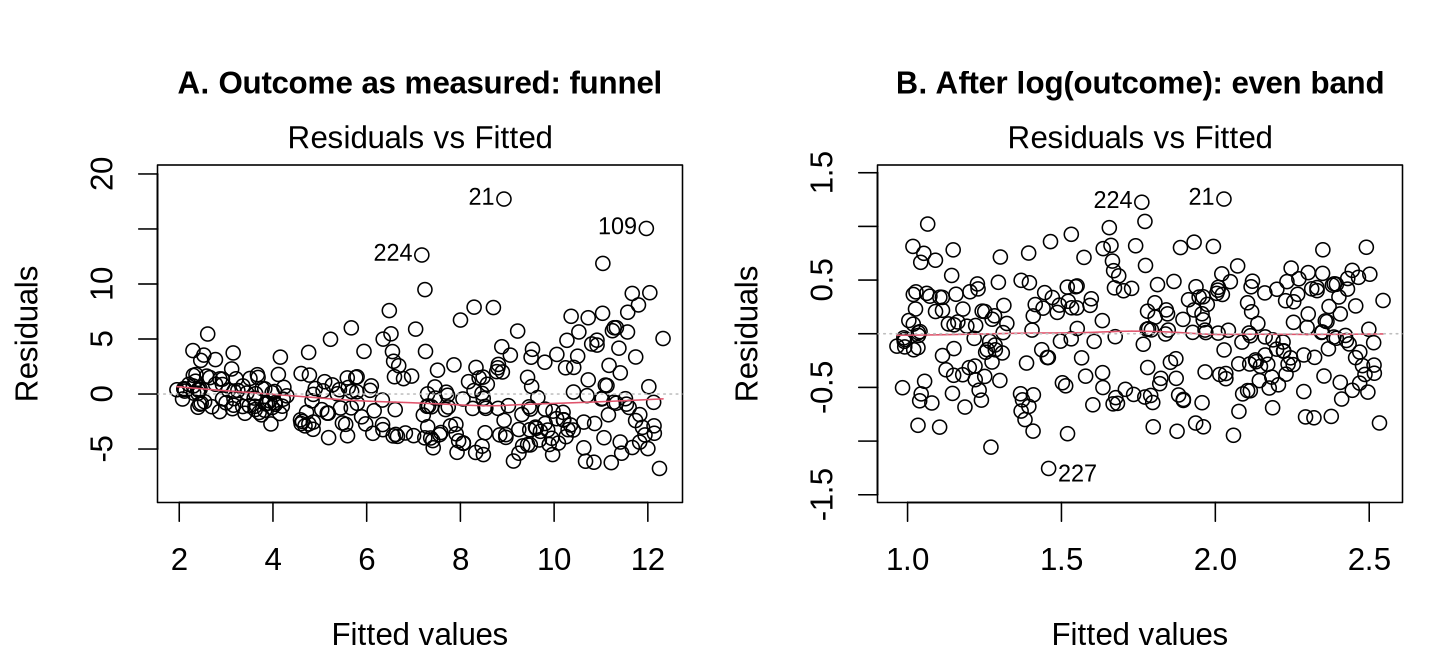
Because the blood pressure model passed every check, Worked Example 3.3 uses simulated data, while Worked Examples 3.4 and 3.5 apply two of the responses to the blood pressure model as checks. The most common response to a funnel is to model the logarithm of a positive, right-skewed outcome. Worked Example 3.3 shows this with simulated cost data; watch how the variance test changes and how the coefficient on the log scale becomes a percentage change.
Costs, lengths of stay and many biomarker concentrations are positive, right-skewed, and more variable when they are larger. Modelling the logarithm of such an outcome often removes the funnel. The simulated example in Figure 3.8 behaves in this way.
library(car)   # for ncvTest()
set.seed(411)
x    <- runif(300, 0, 10)
cost <- data.frame(x, y = exp(1 + 0.15 * x + rnorm(300, sd = 0.45)))
model_cost    <- lm(y ~ x, data = cost)        # outcome as measured
model_logcost <- lm(log(y) ~ x, data = cost)   # log-transformed outcome
ncvTest(model_cost)
ncvTest(model_logcost)
coef(model_logcost)
exp(coef(model_logcost)["x"]) # multiplicative change per unit of xThe variance test moves from p = 1.7 × 10⁻¹⁴ to p = 0.55 after the transformation. The coefficient on the log scale, 0.159, is interpreted after exponentiation, the step that reverses the logarithm: the last line of the output, exp(coef(model_logcost)["x"]), prints 1.17, so each one-unit increase in x multiplies the geometric mean of the outcome by 1.17, a 17% increase. The general rule is that a coefficient β for a log-transformed outcome corresponds to a percentage change of 100 × (eβ − 1), where e is the mathematical constant, about 2.718, on which natural logarithms are based. Predictions from such a model, transformed back with exp(), estimate the geometric mean of the outcome, which for a skewed outcome lies close to the median and below the arithmetic mean. A transformation requires an outcome that is always positive; for outcomes with zeros or negative values, sandwich standard errors are the simpler choice.
The transformation removed the funnel and changed how the coefficient is read, from a difference to a percentage change. When the outcome cannot be logged, or its original scale should be kept, sandwich standard errors are the alternative. Worked Example 3.4 applies them to the blood pressure model as a check on the equal-variance assumption.
Sandwich (heteroscedasticity-consistent, HC3) standard errors, from coeftest(model, vcov = vcovHC(model, type = "HC3")) in the lmtest and sandwich packages, recompute the uncertainty of each coefficient without assuming equal variance. By this we mean that the ordinary standard errors are calculated from a single residual variance that is assumed to apply to everyone, whereas the sandwich method uses the size of each person’s own residual, so it remains valid when the spread of the residuals differs across people. The coefficients themselves do not change, because only the measure of their uncertainty is recalculated. For the blood pressure model, the sandwich standard error for smoking is 0.881 mmHg against 0.844 mmHg from summary(), and the other standard errors change by similar small amounts. When the two sets of standard errors agree this closely, the equal-variance assumption is not affecting the conclusions.
Close agreement between the two sets of standard errors confirms the visual and formal checks of 4.1. The usual first response to a curve, a squared term, has a side effect that links back to 4.2: a predictor and its square are strongly correlated. Worked Example 3.5 adds a squared age term to the blood pressure model and shows the effect on the standard error of age and how it is avoided.
When the squared age term is added to the blood pressure model, age and age² are almost perfectly correlated (r = 0.98), because every age lies between 18 and 87, far from zero. Table 3.7 compares the models.
Table 3.7. The age coefficient and its standard error with and without a squared age term, and with age centred at its mean before squaring.
| Model | Age estimate (SE) | t value for age | VIF for age; for age² | Squared term |
|---|---|---|---|---|
| Straight line in age (Activity 3.2) | 0.427 (0.024) | 18.1 | 1.08; none | None |
| Age + age² | 0.505 (0.122) | 4.1 | 29.0; 28.9 | p = 0.51 |
| Age centred at 45.2 + its square | 0.428 (0.024) | 18.1 | 1.09; 1.01 | p = 0.51 |
Adding age² raises the standard error of age from 0.024 to 0.122, about five times as large, in line with the square root of its VIF of 29, which vif() prints in its last column as 5.39 for the model with the squared term (question 3 of Activity 3.2); the t value falls from 18.1 to 4.1. The model fits no better (the squared term has p = 0.51), so the response is to drop the squared term and keep the straight-line model. If a curve were needed, the predictor would be centred at its mean before squaring: the centred model fits the data identically, but its VIFs fall to about 1 and the standard error of age returns to 0.024.
Here the squared term costs precision without improving the fit, so the straight line in age is kept. The narrated walkthrough below works through the same sequence on a second dataset, from exploring the variables to responding to problems, as optional practice before the activity.
This walkthrough fits a linear regression and a logistic regression to the Canadian Social Connection Survey and checks the assumptions of each model, in the order an analyst normally works: explore the variables, fit the model, check it, respond to any problems and interpret the results.
Open the Linear and Logistic Regression in R walkthroughActivity 3.2 practises 2.3 to 4.3 on the PHAA survey. Run along to fit the five-predictor model, read its coefficients and fit statistics, and check it with the diagnostic plots, formal tests, Cook’s distance, variance inflation factors and sandwich standard errors, answering three questions along the way.
Text version of the activity: the code of the run-along script, its console output and notes on reading it.
phaa <- read.csv("https://heal-learn.ca/r-activities/data/phaa_survey_clean.csv")   # course data, read from the website
phaa$smoker <- factor(phaa$smoker, levels = c("No", "Yes"))   # "No" = reference
phaa$gender <- factor(phaa$gender, levels = c("Man", "Woman", "Non-binary"))
cc <- na.omit(phaa[, c("systolic_bp", "age", "gender", "smoker", "bmi", "dep_score")])
nrow(cc)                     # people with complete data for the model
model <- lm(systolic_bp ~ age + gender + smoker + bmi + dep_score, data = cc)
summary(model)
round(confint(model), 2) # 95% confidence intervalsReading the output. The Coefficients table gives each estimate, its standard error, the t value and the p-value. genderWoman and genderNon-binary compare each group with men. The last three lines give the residual standard error, R², adjusted R² and the F-test, and the confidence intervals follow.
par(mfrow = c(2, 2))         # four plots on one screen
plot(model)                  # the four diagnostic plots
par(mfrow = c(1, 1))         # back to one plot per screen
model_sq <- lm(systolic_bp ~ age + I(age^2) + gender + smoker + bmi + dep_score, data = cc)
anova(model, model_sq)       # linearity: does a squared age term help?
bptest(model)                # equal spread (Breusch-Pagan test)
shapiro.test(residuals(model)) # normality of the residualsThe four plots appear in the Plots pane and match Figure 3.3. The squared-age comparison, the Breusch-Pagan test and the Shapiro-Wilk test follow.
cooks <- cooks.distance(model)
sum(cooks > 4 / nrow(cc))    # rows above the 4/n screening line
round(max(cooks), 3)         # the largest Cook's distance
vif(model)                   # collinearity (values near 1 are good)
round(coeftest(model, vcov = vcovHC(model, type = "HC3"))[, 1:2], 3) # sandwich SEsFor a categorical predictor with more than one indicator, vif() reports a generalised VIF (GVIF) in the first column, which is read like an ordinary VIF for a term with one degree of freedom. The last column, GVIF^(1/(2*Df)), is on the square-root scale: it is the factor by which the standard error is inflated, so square it before comparing it with the usual VIF cut-offs of 5 and 10 (for age here, 1.040 in the last column is the square root of its GVIF of 1.08). It lets a variable with several indicators, such as gender, be compared with the others. The last line gives sandwich (HC3) standard errors, which do not assume equal variance.
Answer each question from your own output, as on the midterm: find the number, say what it means, judge the check.
1. Using summary(model) and confint(model), interpret the coefficients for age, smokerYes and genderWoman, attaching units to each and naming the comparison each coefficient makes. What proportion of the variance in systolic blood pressure do the predictors explain, after a penalty for the number of predictors?
2. Based on the diagnostic plots, the squared-age comparison, bptest() and shapiro.test(), would you continue to use this linear model? Name the assumption each check addresses and cite the evidence. Should the 35 people above the 4/n line for Cook's distance be removed?
3. Run your own code: after line 22 of the script, type summary(model_sq) and vif(model_sq) and run them. Identify the problem the diagnostics reveal, describe its effect on the standard error of the age coefficient by comparing the two models, and state what you would do about it.
The output of the activity matches Table 3.3, Figure 3.3 and the results in Table 3.4. This section has fitted a multivariable linear regression, read its output, checked its assumptions and described the responses when a check fails. The knowledge check that follows reviews these points.
lm(), each coefficient is an adjusted difference in the mean outcome, and a complete interpretation names four things: its size in the units of the outcome, the comparison it makes, what is held constant and its uncertainty. For a numeric predictor the comparison is per one-unit increase, as in "each additional year of age is associated with a mean systolic blood pressure 0.43 mmHg higher (95% CI 0.38 to 0.47), holding gender, smoking, BMI and depression score constant." For a categorical predictor each indicator compares its category with the reference category, so smokers averaged 6.15 mmHg higher than non-smokers of the same age, gender, BMI and depression score, and genderWoman (−0.34 mmHg) compares women with men, not with everyone else; check the reference in the code (factor(..., levels = ) or relevel()) before you write. The intercept is the prediction when every numeric predictor is 0 and every factor is at its reference category, which often lies outside the data; centring a predictor (for example, age − 50) moves its zero into the data and changes the intercept but not the slope. For a predictor entered as ln(x + 1), the coefficient is the change per one-unit increase in ln(x + 1), which means multiplying (x + 1) by about 2.72, and the predicted difference between two values, β × [ln(x2 + 1) − ln(x1 + 1)], is obtained in R in one line, as 2.3.3 shows.summary() coefficient table carries its own test of whether that coefficient differs from zero. The t value is the estimate divided by its standard error, so it says how many standard errors the estimate lies from zero, and Pr(>|t|) is the probability of an estimate at least that far from zero if the true coefficient were 0. The 95% confidence interval from confint() is approximately the estimate ± 1.96 standard errors and shows both the size of the effect and how precisely it is estimated: for smoking, confint() prints 4.49 to 7.80 mmHg, roughly the estimate plus or minus two standard errors. These formulas explain what the printed numbers measure (the printed t value of 7.28 says that the smoking estimate lies about seven standard errors from zero), and you can read significance from the interval, because a 95% interval that excludes 0 goes with p < 0.05. An interval that includes 0, such as −1.58 to 0.90 for women against men, means the data are compatible with no difference; it does not prove that there is none, so word it as "no clear evidence of a difference".summary() describe the model as a whole. R² is the share of the variation in the outcome that the predictors explain (0.414 for the blood pressure model), and adjusted R² applies a penalty for each predictor (0.409); because R² always rises as predictors are added, adjusted R² is the statistic to give when a question asks for the variance explained after penalising for unnecessary predictors, or when models of different sizes are compared. The residual standard error (8.70 mmHg) is the typical distance between an observed value and the model's prediction, in the units of the outcome, and the F-test (F = 92.7 on 6 and 788 df) asks whether the predictors together explain more than chance. The analysis of variance table printed by anova(model) shows where these numbers come from: the residual Mean Sq is the MSE (75.6), and its square root is the residual standard error; R² = 1 − SSE ÷ SST compares sums of squares, whereas adjusted R² = 1 − MSE ÷ MST compares mean squares, which is how it penalises each extra predictor. Read the values themselves from summary(), and avoid the usual slip of reporting the Multiple R-squared when a question asks for the variance explained after a penalty for the number of predictors.plot(model) gives four panels to check them: an even band with a flat smoother in Residuals vs Fitted (linearity), points along the diagonal in Q-Q Residuals (normality), a flat line in Scale-Location (equal variance) and no points beyond the Cook's distance contours in Residuals vs Leverage (influence). The formal tests back the plots up: a squared term compared with anova() for linearity, bptest() for equal variance and shapiro.test(residuals(model)) for normality, where a small p-value signals a problem; the blood pressure model passed all three (p = 0.51, 0.58 and 0.62). Read the panels together and let them lead, because in a large sample the Shapiro-Wilk test can reject departures too small to matter, while in a small sample it can miss ones that do. When you describe a panel in an exam, say what you see, which assumption it checks and whether that assumption is met.cooks.distance(model), measures how far the coefficients would move if one observation were removed: values above 0.5 warrant investigation and values above 1 are serious, whereas the 4/n line is only a liberal screen that flags a few per cent of rows in almost any dataset, so crossing it is not a reason to delete anyone (the largest value here was 0.061). The variance inflation factor, VIF = 1 ÷ (1 − R²j) from vif(model), shows how well a predictor is explained by the other predictors: 1 means no collinearity, above 5 is concerning and above 10 is serious. Collinearity does not bias a coefficient, but it inflates its standard error by about √VIF, which widens the confidence interval and shrinks the t value. When an exam shows two models, compare the standard errors that R prints: adding age² raised the VIF for age to 29 and its standard error from 0.024 to 0.122, about 5 times as large, in line with √29 = 5.4, so its t value fell from 18.1 to 4.1.crPlots() calls for a squared term or a spline for that predictor, compared with the straight-line model using anova(old, new); a funnel with a rising Scale-Location line calls for modelling the logarithm of a positive, right-skewed outcome, lm(log(y) ~ x), or keeping the model and using sandwich standard errors, coeftest(model, vcov = vcovHC(model, type = "HC3")). An influential point is first checked for an entry error, and the model is then fitted with and without it and both results are reported; a collinear squared term is dropped if it does not improve the fit, or the predictor is centred before it is squared. Some failures mean the model itself is wrong: two parallel bands of residuals point to a 0/1 outcome that needs logistic regression, counts need a Poisson or negative binomial model, and clustered observations need a mixed model or GEE. Two last reminders: a coefficient for a log-transformed outcome is read as a percentage change of 100 × (eβ − 1), which R prints with 100 * (exp(coef(model)) - 1), and a modest Q-Q departure in a large sample, with the other panels clean, usually needs no change at all.1. A study of university students fits lm(dep_score ~ sleep_c + residence), where dep_score is a depression score in points, sleep_c is hours of sleep per night minus 7, and residence has three categories with "With family" as the reference category. The estimates are: intercept 9.2, sleep_c −0.8, residenceAlone 2.1 and residenceShared 0.6. Which interpretation is correct?
2. In a linear model for systolic blood pressure (mmHg) fitted to 600 adults, R prints the results below for waist circumference (cm), which is adjusted for the other predictors in the model. What do the t value and the 95% confidence interval show?
confint() (0.11 to 0.89 mmHg per cm). The interval gives the range of adjusted differences that are consistent with the data, and because it lies entirely above 0, p is below 0.05. Option a is the tempting misreading: the t value is a distance from zero measured in standard errors, and the p-value is the probability of an estimate at least this far from zero if the true coefficient were 0, not the probability that it is 0. Option b turns a difference in mean blood pressure into a fixed effect in every adult, and option c is wrong because the interval excludes 0 and shows the plausible size of the association. (Section 2, 3.1 Testing Each Coefficient; Objective 3.1)3. A linear model for a physical-function score (points) is fitted to 205 adults with age, BMI and a three-category activity level as predictors, and the bottom of summary(model) reads as shown below. Which statement gives the proportion of the variance in the score that the predictors explain after penalising the model for the number of predictors?
4. A linear model is fitted to 5,000 people. The Shapiro-Wilk test of the residuals gives p = 0.01, the Q-Q plot shows the points on the diagonal apart from a slight bend at the upper end, and the other three diagnostic panels look adequate. What is the best conclusion about the normality assumption?
5. A linear model for a lung-function score includes age in years. To check for a curve, a squared age term is added. The standard error of the age coefficient rises from 0.010 to 0.040, the variance inflation factors are 16.2 for age and 16.0 for age², and the squared term has p = 0.62. Which statement is correct?
6. A linear model for annual health care cost (dollars), a positive and right-skewed outcome, shows a funnel that widens from left to right in the Residuals vs Fitted plot, a rising line in the Scale-Location plot, and ncvTest() p < 0.001. Which first response is most appropriate?
7. A cardiac rehabilitation programme models the six-minute walk distance (metres) of 412 patients. Model A includes centred age, sex, diabetes and the number of other chronic conditions (conds). Model B adds the number of prescribed medications (meds), which is correlated 0.94 with conds; in Model B, meds has a coefficient of 0.01 m (p = 1.00). Which reading of the output below is correct?
conds in each model, the VIFs and the p-value for meds. Collinearity between two measures of much the same thing does not bias a coefficient (−13.97 against −13.98) but inflates its standard error by about √VIF, here from 2.13 to 6.23, so its confidence interval widens and its t value shrinks. A VIF above 5 is concerning and one above 10 is serious, so values of 9.14 and 9.16 are a clear warning, which rules out option d. Because meds adds nothing to the model (p = 1.00), the usual response is to keep the variable with the stronger rationale, conds, and drop meds; combining the two counts into one index, or keeping both and reporting the wider intervals, are the alternatives. Option a is the tempting error, since collinearity costs precision rather than causing bias, and option c removes the better variable because of a problem that adding meds created. (Section 2, 4.2 Influential Observations and Collinearity, Table 3.4 and Worked Example 3.5; Objective 4.2)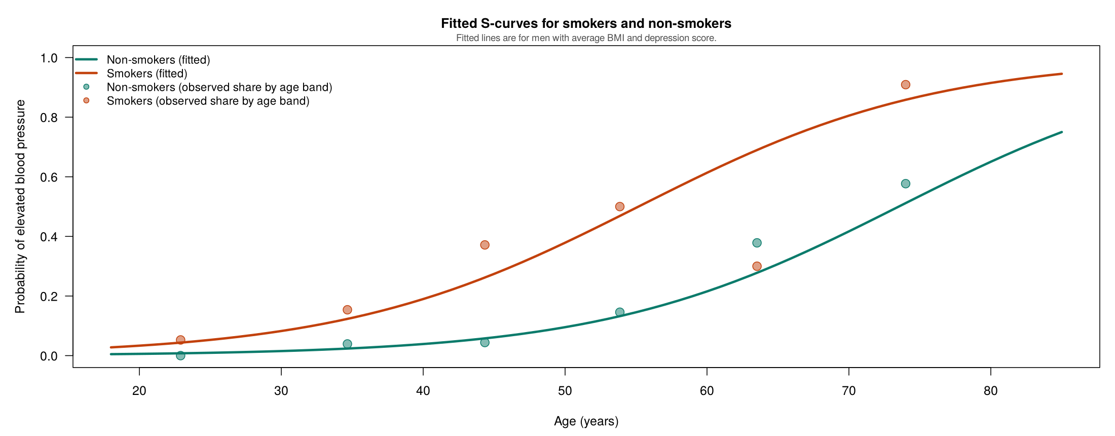
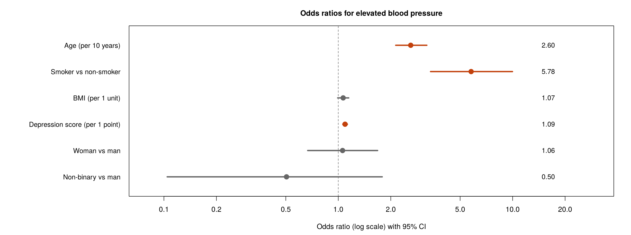
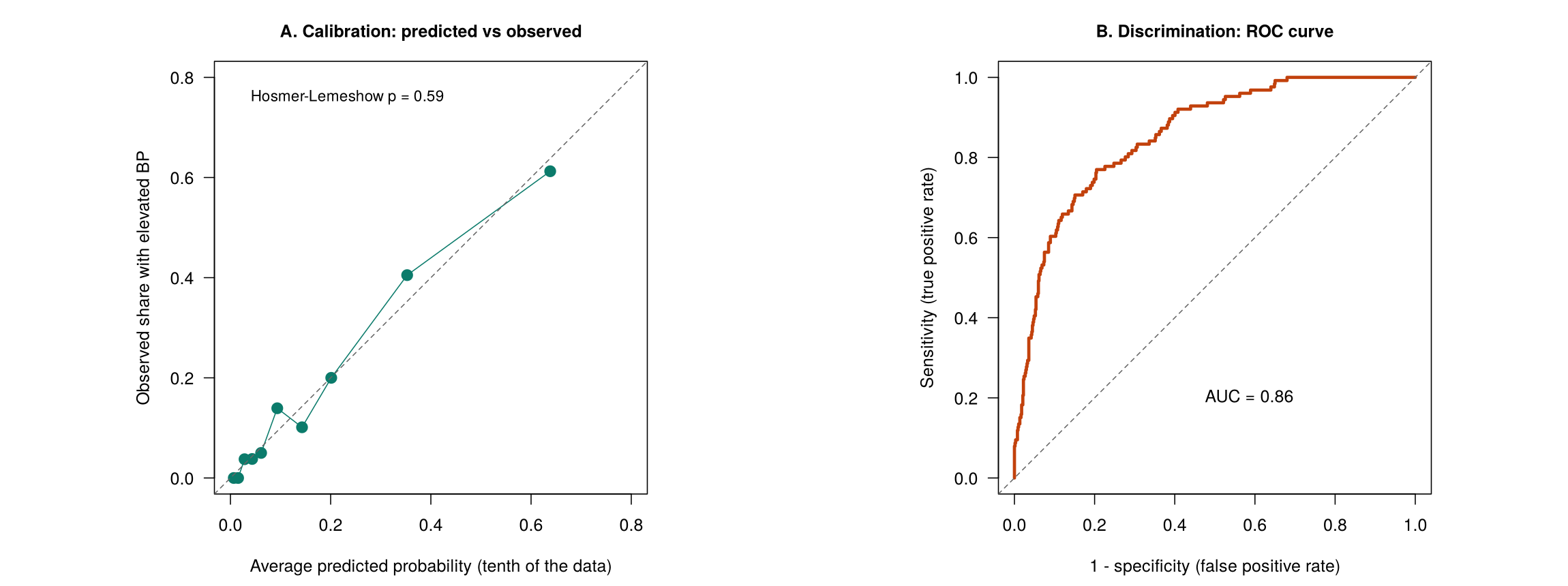
This section models a binary outcome, elevated blood pressure (a systolic reading of 120 mmHg or more), with logistic regression. It explains why a straight-line model does not suit such an outcome, how probabilities, odds and log odds are related, how to fit a logistic model in R and read its coefficients as odds ratios, how predicted probabilities show what an odds ratio means, and how the model is checked for events per coefficient, linearity, overall fit, calibration and discrimination. It uses the same five predictors as Section 2 and the 795 PHAA participants with complete data, of whom 126 have elevated blood pressure.
glm(..., family = binomial) and interpret its exponentiated coefficients as odds ratios.A binary outcome takes only two values, coded 1 for the event (elevated blood pressure) and 0 otherwise. The average of such a 0/1 variable is the proportion of people with the event, so a regression of a binary outcome is really a model for the probability of the event. A linear regression fitted to such an outcome, however, breaks three rules at once. First, a straight line has no upper or lower limit, so it can predict values below 0 or above 1, which cannot be probabilities. Second, its residuals cannot be normally distributed. Because every observed outcome is either 0 or 1, for any fitted value p̂ a residual can only be 1 − p̂ (for a person with the event) or −p̂ (for a person without it). Instead of a smooth bell-shaped spread, the residuals therefore fall on two lines, which shows as two parallel bands in the Residuals vs Fitted plot.
Third, the variance of a 0/1 outcome, p(1 − p), changes with the predicted probability. By this we mean that the outcome is most variable when the probability is near 0.5 and least variable when it is near 0 or 1, so the spread of the residuals cannot be the same for everyone. As a result, the equal-variance assumption fails and the standard errors and tests are unreliable. These problems come from the type of outcome rather than from the particular data, so a larger sample does not remove them. Nor do the usual repairs help: a log transformation cannot be applied (the logarithm of 0 is undefined), and sandwich standard errors, while they correct the standard errors, cannot turn a negative prediction into a probability. Logistic regression avoids all three by modelling the probability through an S-shaped curve that always stays between 0 and 1.
Click each of the three cards below: the first sums up the three problems, and the other two introduce the logit transform and the odds ratio, which the rest of this section develops.
Worked Example 3.6 fits a linear model to the 0/1 outcome anyway, to show how each of the three problems appears in R output; for each piece of evidence, note the problem it reveals and the number that shows it.
lm() Is Fitted to a 0/1 OutcomeElevated blood pressure was coded 1 (yes) or 0 (no) and fitted with lm() using the same five predictors as the logistic model, for the same 795 people. Each coefficient is then a difference in the probability of the outcome; for example, the smoking coefficient of 0.23 says that smokers are 23 percentage points more likely to have elevated blood pressure. The checks in Table 3.8 show why this model cannot be trusted.
Table 3.8. Evidence from a linear model fitted to the 0/1 outcome, and what each piece of evidence shows.
| Output | Result | Problem it shows |
|---|---|---|
summary(fitted(lpm)); sum(fitted(lpm) < 0) | Fitted values from −0.28 to 0.82; 153 people have a fitted value below 0 | Out-of-range predictions: a probability cannot be negative. |
Breusch-Pagan test, bptest(lpm) | BP = 152.3 on 6 df, p < 0.001 | Unequal variance: the variance of a 0/1 outcome is p(1 − p), which changes with the predicted probability, so the standard errors and tests are unreliable. |
shapiro.test(residuals(lpm)) and the Residuals vs Fitted plot | W = 0.865, p < 0.001; the residuals form two parallel bands | Non-normal residuals: for any fitted value p̂, a residual can only be 1 − p̂ or −p̂. |
Each piece of evidence names a problem, explains why it matters and points to a number in the output. Together they lead to the decision to switch to a logistic regression with glm(..., family = binomial(link = "logit")), whose predicted probabilities always lie between 0 and 1.
The output therefore points to a different model. Logistic regression is built on the odds and the log odds of the outcome, which the next subsection defines.
A probability and an odds are two different ways of describing how likely an event is. A probability compares the number of people with the event with everyone in the group, whereas an odds compares the number of people with the event with the number of people without it. Formally, for an outcome with probability p, the odds are p ÷ (1 − p), the probability that the event happens divided by the probability that it does not. The two scales agree on order, so a higher probability always means higher odds, but they are not the same number. A probability of 0.5 corresponds to odds of 1, a probability of 0.2 to odds of 0.25, and a probability of 0.8 to odds of 4. In a 2 × 2 table, each group’s odds are its number of events divided by its number of non-events: among smokers, 48 of 135 have elevated blood pressure, so 48 out of 135 is their probability and 48 to 87 their odds. Labelling every number as a probability or an odds before interpreting it avoids the most common slip. The odds ratio (OR) divides the odds in one group by the odds in another. By this we mean that it compares two groups by asking how many times larger the odds are in one group than in the other, in the same way that a difference in means compares two groups for a numeric outcome. R reports the crude odds ratio for smoking as the exponentiated coefficient of a logistic regression with smoking as its only predictor: exp(coef(glm(elevated_bp ~ smoker, family = binomial, data = phaa))) prints 4.02 for smokerYes, and 0.137, the odds among non-smokers, for the intercept. Smokers therefore have about four times the odds of elevated blood pressure of non-smokers. An odds ratio of 1 means no association, a value above 1 higher odds and a value below 1 lower odds. Because an odds ratio compares odds rather than probabilities, it is described as “times the odds”, not “times as likely”; 5.4 shows how far apart the two can be.
The log odds, or logit, is the natural logarithm of the odds, ln[p ÷ (1 − p)]. The reason for taking this extra step is the range of values each scale allows. A probability is trapped between 0 and 1, and the odds remove the upper limit but cannot fall below 0. Taking the logarithm removes the lower limit as well: odds below 1 become negative log odds, odds of 1 become a log odds of 0, and odds above 1 become positive log odds. As a result, the log odds ranges from −∞ to +∞, which allows it to be modelled with a straight line, because no value of the predictors can push the line to an impossible value. Logistic regression is therefore a linear model, but for the log odds of the outcome rather than for the outcome itself. Equation 3.2 gives the logistic regression model on the log-odds scale and, by reversing the logit, on the probability scale.
Interactive 3.3 shows a model with one predictor in both forms at once. Move the intercept and slope sliders and watch the straight line on the log-odds scale become an S-shaped curve on the probability scale; note that the odds ratio per unit of X depends only on the slope, while the change in probability depends on where you start.
Move the sliders to change the intercept (β₀) and slope (β₁). The left panel shows the model on the log-odds scale, where it is a straight line; the symbol η (the Greek letter eta) stands for this straight-line part of the model, β₀ + β₁X, which is often called the linear predictor. The right panel converts the same model into probabilities with the logistic function, written σ (sigma), so that p = σ(η) traces an S-shaped curve that always stays between 0 and 1. The S-curve’s steepness is set by β₁, and its midpoint, the value of X at which the probability equals 0.5, is −β₀/β₁.
The S-curve is why logistic coefficients are read as odds ratios rather than as changes in probability: a one-unit change in a predictor multiplies the odds by the same amount everywhere, but moves the probability by different amounts depending on the starting point. The next subsection fits the model to the PHAA data.
The model is fitted with glm(elevated_bp ~ age + gender + smoker + bmi + dep_score, family = binomial, data = cc), where elevated_bp is a factor with levels "No" and "Yes", so that R models the probability of "Yes". The coefficients are on the log-odds scale, and exp(cbind(OR = coef(logit), confint(logit))) turns them into odds ratios with 95% confidence intervals.
Each coefficient is the change in the log odds for a one-unit increase in its predictor, holding the other predictors constant, and exponentiating it, eβ, turns it into an adjusted odds ratio. Table 3.9 lists the coefficients of the model, the odds ratios obtained from them, and an interpretation of each.
Table 3.9. Coefficients and odds ratios with 95% confidence intervals from the five-predictor logistic regression, with an interpretation of each.
| Predictor | Coefficient (log odds) | Odds ratio (95% CI) | Interpretation |
|---|---|---|---|
| Age (per year) | 0.096 | 1.10 (1.08 to 1.12) | Each additional year multiplies the odds by 1.10; over 10 years, the odds ratio is 2.60, which exp(10 * coef(logit)["age"]) prints. |
| Woman vs man | 0.057 | 1.06 (0.67 to 1.68) | No clear difference. |
| Non-binary vs man | −0.684 | 0.50 (0.10 to 1.79) | Very uncertain, because only 3 of the 27 non-binary participants have elevated blood pressure. |
| Smoker vs non-smoker | 1.754 | 5.78 (3.38 to 9.98) | Smokers have 5.8 times the odds of non-smokers with the same age, gender, BMI and depression score. |
| BMI (per unit) | 0.064 | 1.07 (0.99 to 1.15) | The interval just includes 1 (p = 0.083). |
| Depression score (per point) | 0.089 | 1.09 (1.06 to 1.13) | Each additional point multiplies the odds by 1.09. |
The adjusted odds ratio for smoking (5.78) is larger than the crude odds ratio (4.02 in all 798 people with a reading, and 4.03 in the 795 people with complete data whom the model uses). This change should not be read as evidence of confounding. Smokers and non-smokers in the model have almost the same average age (45.5 and 45.1 years), so age cannot be distorting the comparison between them in the way a confounder would. Yet adding age alone raises the odds ratio from 4.03 to 5.28. This happens because an odds ratio changes when strong predictors of the outcome are added to the model, even when they are not confounders, a property known as non-collapsibility. By this we mean that the odds ratio for a whole group mixing people of different ages is not simply an average of the odds ratios within each age, and it is usually closer to 1. Adding age therefore changes the question from a comparison across a mixed population to a comparison among people of the same age, and that comparison gives a larger odds ratio. A linear regression coefficient does not behave in this way, which is why the same reasoning about confounding cannot be carried over to logistic models unchanged. Part of the change also reflects adjustment for BMI, which Section 4 treats as a mediator.
Expand the four panels below for how a dichotomous, a continuous and a multi-level categorical predictor are interpreted, including Equation 3.3 for an odds ratio over a change of several units, and for what the intercept means.
For a dichotomous predictor (coded 0/1), the coefficient β represents the log odds ratio comparing the group coded 1 to the group coded 0, adjusted for all other variables. The odds ratio is OR = eβ, where e (about 2.718) is the base of the natural logarithm; raising e to the power β reverses the logarithm and turns the log odds ratio back into an odds ratio. For example, in this section's model βsmoking = 1.754, and exp(coef(logit)) prints the odds ratio as 5.78, meaning that the odds of elevated blood pressure are 5.78 times as high for smokers as for comparable non-smokers.
For a continuous predictor, β represents the change in the log odds for each 1-unit increase in the predictor. The OR = eβ gives the multiplicative change in odds per unit increase, that is, the number by which the odds are multiplied each time the predictor rises by one unit; an OR of 1.10 means the odds rise by 10% with each additional unit. Equation 3.3 gives the OR for any change from x1 to x2:
For example, in this section's model βage = 0.0957, and R gives the OR per 10-year increase in age in one line, exp(10 * coef(logit)["age"]), which prints 2.60, the odds ratio for a 10-year difference in age.
Categorical predictors with more than two levels are represented using indicator (dummy) variables. One category serves as the baseline/reference, and each coefficient represents the log OR comparing that category to the reference. To judge whether the categorical variable as a whole is associated with the outcome, all of its indicator variables are tested together, using a multi-degree-of-freedom Wald test or an LRT comparing models with and without the entire set of indicator variables. A joint test is needed because each separate coefficient depends on which category was chosen as the reference.
The intercept (β0) represents the logit of the probability of the outcome when all predictors equal zero. On the probability scale, this is: p = 1/(1 + e−β0). The intercept is often not substantively meaningful (e.g., if age = 0 is not a plausible value), but it is essential for computing predicted probabilities. Note that effects on the probability scale are non-linear: the same change in a predictor produces different changes in probability depending on the baseline values of all predictors.
The panel on continuous predictors matters for questions about age: odds ratios combine by multiplication, so the odds ratio for ten years is e10β, which R prints as 2.60, not ten times the one-year odds ratio of 1.10. Odds ratios are hard to translate into risks, and the next subsection addresses this with predicted probabilities.
The model can predict the probability of the outcome for any combination of predictor values. In R, predict(logit, newdata = ..., type = "response") returns probabilities, because type = "response" asks R to apply the probability form of Equation 3.2. Comparing two people who differ in one predictor only shows what an odds ratio means for risk. The ratio of their two predicted probabilities is a risk ratio, that is, how many times as likely one person is to have the outcome as the other. It differs from the odds ratio because the odds and the probability are different scales. When an outcome is rare, the probability of not having it is close to 1 for everyone, so the odds, p ÷ (1 − p), are almost the same number as the probability, and the odds ratio and risk ratio nearly agree. When the outcome is common, the odds grow much faster than the probability as p rises, so the odds ratio lies further from 1 than the risk ratio. For this reason the two are similar only for an outcome that affects fewer than about 10% of people. When the outcome is common, an odds ratio of 5.8 should therefore never be described as 5.8 times the risk. Worked Example 3.7 predicts the probability of elevated blood pressure for one man as a smoker and as a non-smoker; compare the ratio of his two probabilities with the adjusted odds ratio of 5.78.
For a 50-year-old man with a BMI of 21 and a depression score of 21, p <- predict(logit, newdata = two_men, type = "response") gives a predicted probability of elevated blood pressure of 0.0974 if he does not smoke and 0.3842 if he smokes. Converted to odds, p ÷ (1 − p), and divided, the two probabilities give back 5.78, the adjusted odds ratio. The ratio of the probabilities, the risk ratio, which p[2] / p[1] prints as 3.94, is smaller. The odds ratio is larger than the risk ratio because elevated blood pressure is common; for an outcome affecting fewer than about 10% of people, the two are similar. Predicted probabilities like these are often the clearest way to explain a logistic model to a general audience.
Reporting the two probabilities alongside the odds ratio avoids the most common misreading of a logistic model. With the model fitted and interpreted, the next subsection checks whether the data can support it.
Logistic regression has its own checks in place of the normality and equal-variance checks of the linear model. Table 3.10 sets out seven checks, how each is carried out in R and the result for this model. The first four parallel the checks of the linear model, and the last three, overall fit, calibration and discrimination, describe how well the model works as a whole; 6.2 takes up calibration and discrimination.
Table 3.10. Checks of the five-predictor logistic regression, how each is carried out in R, and the result for this model.
| Check | What it asks | How in R | Result for this model |
|---|---|---|---|
| Events per coefficient | Are there enough events (about 10 or more per estimated coefficient)? | table(cc$elevated_bp) | 126 events for 6 coefficients, 21 per coefficient |
| Linearity on the log-odds scale | Does a continuous predictor need a curve? | Add a squared term; anova(..., test = "Chisq") | Squared age: p = 0.43 |
| Collinearity | Are the predictors too strongly correlated? | vif() | All below 1.14 |
| Influence | Does any observation change the results much? | cooks.distance() | Largest value 0.065 |
| Overall fit | Do the predictors improve on a model with none? | Likelihood ratio test against glm(y ~ 1) | Deviance drop 199.4 on 6 df, p < 0.001 |
| Calibration | Do predicted probabilities match observed shares? | ResourceSelection::hoslem.test() | χ² = 6.50 on 8 df, p = 0.59 |
| Discrimination | Does the model separate people with and without the outcome? | pROC::auc() | AUC = 0.86 |
The first check is sample size. In logistic regression the information about each coefficient comes mainly from the people with the less common outcome, because the model learns how the predictors differ between those who have the event and those who do not, and the smaller of the two groups limits that comparison. A common guide therefore asks for at least 10 events per estimated coefficient, where the events are the less common outcome rather than all the people, and a categorical predictor with k categories uses k − 1 coefficients. This model has 126 events among 795 people and six coefficients besides the intercept, and the line of Activity 3.3 that divides one by the other prints 21 events per coefficient, which is enough. Linearity is now judged on the log-odds scale: adding a squared term for age and comparing the two models with anova(..., test = "Chisq") gives p = 0.43, so the straight line in age stays.
With too few events per coefficient, logistic regression estimates become unstable and their confidence intervals very wide. The survey's hypertension variable, with 23 cases, would support only about two predictors. A related problem, called separation, occurs when a predictor category has no events at all, or only events. In that case the odds in the category are 0 or infinite, so the log odds the model is trying to estimate has no finite value, and the estimate for that category then grows without limit. In practice R stops at a very large coefficient with an enormous standard error, which is the sign to look for. The non-binary group, with 3 events among 27 people, shows the milder version of this problem: its odds ratio of 0.50 has a confidence interval from 0.10 to 1.79.
Overall fit is judged with the deviance, which measures how far a model is from fitting the data perfectly. It plays a role similar to the residual sum of squares in linear regression: a smaller deviance means that the model’s predicted probabilities sit closer to the outcomes people actually had. A deviance on its own has no fixed meaning, however, because its size depends on the number of people and the outcome; it is judged only against the deviance of another model fitted to the same people. The likelihood ratio test makes that comparison. It compares the deviances of two nested models fitted to the same people, where nested means that the smaller model is the larger one with some terms removed, and it asks whether the drop in deviance from adding those terms is larger than chance would produce. For example, here the deviance falls from 695.1 for the model with no predictors to 495.6 for the full model, a drop of 199.4 on 6 degrees of freedom (p < 0.001), so the predictors clearly help. McFadden’s pseudo-R², which R gives as 1 - logit$deviance / logit$null.deviance = 0.29, summarises the improvement on a scale from 0 to 1, but it is not the share of variance explained and is usually much lower than R² from a linear model.
Individual terms are tested in two ways. Each row of summary(logit) gives a Wald test, z = estimate ÷ standard error, which for an indicator compares one category with the reference category only. A categorical predictor as a whole is tested with a likelihood ratio test that compares the models with and without all of its indicators. Worked Example 3.8 compares the two tests for gender; watch which question each test answers, and how the result is combined with the causal diagram to decide whether gender stays.
The Wald test. Each row of summary(logit) gives a Wald test: z = estimate ÷ standard error, with its p-value in Pr(>|z|). For gender, the two rows test separate comparisons with the reference category, men: genderWoman has z = 0.24 (p = 0.81) and genderNon-binary has z = −0.97 (p = 0.33). A single indicator's p-value compares one category with the reference category only, and it changes if a different reference category is chosen, so it cannot say whether gender as a whole matters.
The likelihood ratio test. Gender is one variable represented by two indicators, so it is tested as a whole by comparing the full model with the same model without gender, fitted to the same 795 people: anova(logit_no_gender, logit, test = "LRT") (or test = "Chisq"). The test statistic is the drop in deviance, G² = deviance of the smaller model − deviance of the larger model, which anova() prints in its Deviance column as 1.25, compared with a χ² distribution whose degrees of freedom equal the number of terms removed (2). Here p = 0.53, so gender as a whole adds little to the fit. The likelihood ratio test has better statistical properties than the Wald test and is preferred when the two disagree.
The decision. A non-significant test is not a reason to remove gender. The causal diagram in Section 4 treats gender as a confounder of the effect of smoking, and confounders are retained regardless of statistical significance, because removing a confounder would leave its back-door path open. In these data, dropping gender would barely move the smoking odds ratio (from 5.78 to 5.85), which is consistent with keeping it at little cost in precision. The same reasoning applies when the joint test is significant even though one indicator is not: the variable stays, because its indicators are tested together.
The joint test, not a single indicator’s p-value, judges a categorical predictor, and a confounder stays in the model whatever either test shows. The last two checks ask how well the model’s predictions match the outcomes.
Calibration and discrimination answer two different questions. Calibration asks whether the predicted probabilities match what is observed: do people given a 30% probability have the outcome about 30% of the time? The Hosmer-Lemeshow test, from ResourceSelection::hoslem.test(), splits the data into ten groups by predicted probability and compares the observed and expected numbers with the outcome in each. A non-significant result is the good one, so χ² = 6.50 on 8 df with p = 0.59 gives no evidence of poor calibration. Like other formal tests, the Hosmer-Lemeshow test becomes very sensitive in large samples, so the calibration plot is read alongside it.
Discrimination asks whether the model ranks people with the outcome above people without it. By this we mean that a model that discriminates well gives higher predicted probabilities to the people who turn out to have elevated blood pressure than to those who do not, whether or not those probabilities are exactly right. The area under the ROC curve (AUC), from pROC::auc(), measures this. It is the probability that a randomly chosen person with the outcome has a higher predicted probability than a randomly chosen person without it. For example, if one person with elevated blood pressure and one without it were picked at random many times, a model with an AUC of 0.86 would give the first person the higher predicted probability in about 86% of those pairs. An AUC of 0.5 is no better than chance, 0.7 to 0.8 is acceptable, 0.8 to 0.9 excellent and above 0.9 outstanding, so this model’s 0.86 is excellent. The AUC is neither the share of people classified correctly nor a share of variance explained. A model can do well on calibration and poorly on discrimination, or the reverse, and neither shows that a coefficient is free of confounding. Figure 3.9 shows both properties for the PHAA model.
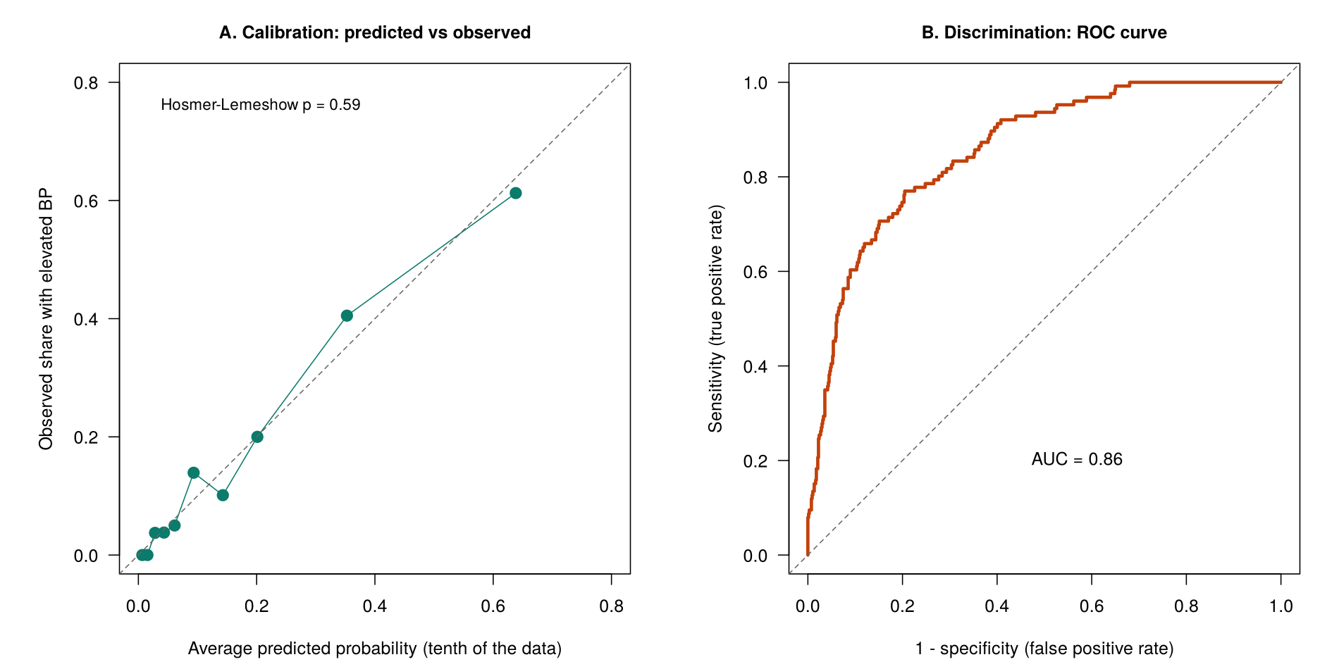
Click each of the three cards below for more on the Pearson χ² goodness-of-fit test, the Hosmer-Lemeshow test, which was designed to get round its limits with continuous predictors, and the ROC curve with the bands used to describe the AUC.
Together, the calibration plot and the ROC curve show that the model’s predicted probabilities are accurate on average and separate people with and without elevated blood pressure well.
Activity 3.3 practises the whole section. Run along to see why a straight line does not suit the yes-or-no outcome, then fit the logistic model, read its odds ratios and predicted probabilities, test gender as a whole and check the model, answering three questions in the style of the midterm along the way.
Text version of the activity: the code of the run-along script, its console output and notes on reading it.
phaa <- read.csv("https://heal-learn.ca/r-activities/data/phaa_survey_clean.csv")   # course data, read from the website
phaa$smoker <- factor(phaa$smoker, levels = c("No", "Yes"))   # "No" = reference
phaa$gender <- factor(phaa$gender, levels = c("Man", "Woman", "Non-binary"))
phaa$elevated_bp <- factor(ifelse(phaa$systolic_bp >= 120, "Yes", "No"),
                           levels = c("No", "Yes"))   # "Yes" = 120 mmHg or more
table(phaa$hypertension)       # the original variable: too few events
cc <- na.omit(phaa[, c("elevated_bp", "age", "gender", "smoker", "bmi", "dep_score")])
table(cc$elevated_bp) # events among the people in the modelThe original hypertension variable has only 23 events, too few for five predictors, so this section uses elevated blood pressure (a systolic reading of 120 mmHg or more): 126 of the 795 people in the model have it.
cc$y01 <- as.numeric(cc$elevated_bp == "Yes")   # 1 = elevated, 0 = not
lpm <- lm(y01 ~ age + gender + smoker + bmi + dep_score, data = cc)
summary(fitted(lpm))           # the predicted "probabilities"
sum(fitted(lpm) < 0)           # how many are below 0?
bptest(lpm)                    # equal spread (Breusch-Pagan test)
shapiro.test(residuals(lpm))   # normality of the residuals
plot(lpm, which = 1)           # Residuals vs Fitted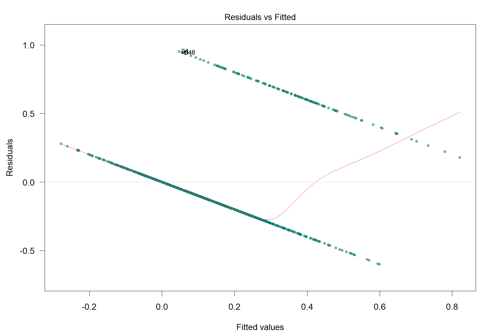
A straight line fitted to the 0/1 outcome predicts values from −0.28 to 0.82, with 153 below 0; the Breusch-Pagan test (BP = 152.33 on 6 df) and the Shapiro-Wilk test (W = 0.865) both give p < 2.2e-16, and the residuals fall on two parallel bands (the plot above).
logit <- glm(elevated_bp ~ age + gender + smoker + bmi + dep_score,
             family = binomial, data = cc)
summary(logit)
round(exp(cbind(OR = coef(logit), confint(logit))), 2)   # odds ratios, 95% CIs
logit_ng <- update(logit, . ~ . - gender)    # the same model without gender
anova(logit_ng, logit, test = "LRT") # gender as a wholeReading the output. The Estimate column is on the log-odds scale, and z value and Pr(>|z|) give a Wald test for each coefficient. confint() on a glm computes profile-likelihood intervals, so R prints "Waiting for profiling to be done..." first. The likelihood ratio test of gender compares the models with and without both gender indicators, fitted to the same 795 people.
round(exp(10 * coef(logit)[["age"]]), 2)     # odds ratio for 10 years of age
two <- data.frame(age = 50, gender = "Man", smoker = c("No", "Yes"),
                  bmi = 21, dep_score = 21)  # differ only in smoking
round(predict(logit, newdata = two, type = "response"), 3)Line 36 prints the odds ratio for ten years of age, 2.6: R multiplies the coefficient by 10 before exponentiating it, which is not the same as ten times the odds ratio of 1.10. The predicted probabilities are for a 50-year-old man with a BMI of 21 and a depression score of 21: 0.097 as a non-smoker and 0.384 as a smoker. Their ratio, the risk ratio, which p <- predict(logit, newdata = two, type = "response"); p[2] / p[1] prints as 3.94, is smaller than the odds ratio of 5.78 because elevated blood pressure is common, so the odds ratio should not be read as a risk ratio.
table(cc$elevated_bp)[["Yes"]] / 6           # events per coefficient
null_model <- glm(elevated_bp ~ 1, family = binomial, data = cc)
anova(null_model, logit, test = "Chisq")     # better than no predictors?
logit_sq <- update(logit, . ~ . + I(age^2))
anova(logit, logit_sq, test = "Chisq")       # linearity on the log-odds scale
round(1 - logit$deviance / logit$null.deviance, 3) # McFadden pseudo R-squaredLine 42 divides the 126 events by the 6 coefficients and prints 21 events per coefficient, above the guide of about 10. McFadden's pseudo-R² (0.287) summarises the improvement on the model with no predictors, but it is not the share of variance explained. The Hosmer-Lemeshow test and the area under the ROC curve are the code you write for question 3.
Answer each question from your own output, as on the midterm: make the decision, give each reason with the number that supports it, and keep the theory and the statistics apart.
1. Lines 19 to 25 fit an ordinary linear model, lm(), to the outcome coded 1 or 0. Based on summary(fitted(lpm)), sum(fitted(lpm) < 0), bptest(lpm), shapiro.test(residuals(lpm)) and the Residuals vs Fitted plot, would you continue to use the lm() function for modelling elevated blood pressure, or would you switch to a binomial logistic regression model using the glm() function? Give each reason with its evidence from the output.
glm(..., family = binomial), because the linear model fitted with lm() is not appropriate for the 0/1 outcome. First, the linear model predicts values outside the range 0 to 1, which cannot be probabilities; the fitted values run from −0.28 to 0.82, and 153 of them are below zero. Second, the variance of a 0/1 outcome is p(1 − p), which changes with the fitted probability, so the constant-variance assumption fails and the standard errors and tests are unreliable; the Breusch-Pagan test gives BP = 152.33 on 6 degrees of freedom, p < 2.2 × 10⁻¹⁶. Third, the residuals cannot be normally distributed, because for any fitted value a residual can take only two values (1 − p̂ or −p̂); the residual plot shows two parallel bands, and the Shapiro-Wilk test gives W = 0.865, p < 2.2 × 10−16.2. Interpret the odds ratio for smokerYes with its 95% confidence interval. The Wald test for genderWoman has a p-value of 0.81, so you ran the likelihood ratio test on lines 32 and 33, which compares the model with the same model fitted to the same people without gender. The causal diagram in Section 4 treats gender as a confounder of the effect of smoking. Based on these results and the theory driving your analysis, should you remove gender from the model? Why or why not?
anova() prints the drop, G² = 1.25, on 2 degrees of freedom, p = 0.53) shows that gender as a whole adds little to the fit, but that is not a reason to drop a confounder.3. Run your own code: after line 47, type hoslem.test(cc$y01, fitted(logit), g = 10) and auc(roc(cc$y01, fitted(logit))). The Hosmer-Lemeshow test checks whether the predicted probabilities match the observed event rates across subgroups (a p-value above 0.05 indicates acceptable fit), and the area under the curve evaluates how well the model separates people with and without the outcome across all thresholds. Interpret the values with respect to how well or unwell your model explains the outcome.
The Hosmer-Lemeshow test and the AUC that you add for question 3 reproduce the values quoted in 6.2. This section has fitted a logistic regression for a binary outcome, read its coefficients as odds ratios and predicted probabilities, and checked the model. The knowledge check that follows reviews these points.
lm() or switch to glm(), state the decision first, then give each reason with three parts: the problem, why it matters and the number in the output that shows it. In the PHAA example the evidence was 153 fitted values below 0 (sum(fitted(lpm) < 0)), a Breusch-Pagan test of BP = 152.3 with p < 0.001, and a Shapiro-Wilk test of W = 0.865 with p < 0.001 alongside the two bands. A large sample does not fix these problems, because they come from the type of outcome, not from the number of people.exp(coef(glm(elevated_bp ~ smoker, family = binomial))). An odds ratio of 4.02 means that smokers have about four times the odds of elevated blood pressure of non-smokers. The most common slip is to read a probability as an odds (48 of the 135 smokers is a probability, not an odds), so label every number as a probability or an odds before you interpret it.glm(..., family = binomial) are on the log-odds scale and must be exponentiated before they are interpreted. exp(cbind(OR = coef(logit), confint(logit))) gives the adjusted odds ratios with their 95% confidence intervals: smokers had 5.78 times the odds of elevated blood pressure of non-smokers with the same age, gender, BMI and depression score (95% CI 3.38 to 9.98). For a numeric predictor the odds ratio is per one-unit increase, and for a change of Δx units the coefficient is multiplied by Δx before it is exponentiated, OR = eβΔx, which R gives in one line: exp(10 * coef(logit)["age"]) prints 2.60 for ten years of age, not 10 × 1.10. Before you interpret anything, check that the outcome is a factor with the event as its second level (levels = c("No", "Yes")), so that R models the probability of "Yes". An odds ratio of 1 means no association, so an interval that includes 1 (BMI, 0.99 to 1.15) gives no clear evidence of one, and your sentence should say "times the odds", not "times as likely".predict(logit, newdata = ..., type = "response"), where type = "response" asks for probabilities (R applies p = 1 ÷ (1 + e−(β0 + β1X1 + …)) for you): a 50-year-old man with a BMI of 21 and a depression score of 21 has a predicted probability of 0.097 as a non-smoker and 0.384 as a smoker. The ratio of those probabilities, the risk ratio, is 3.94, whereas the ratio of their odds is 5.78, the adjusted odds ratio. The odds ratio is larger because elevated blood pressure is common; the two are similar only for an outcome affecting fewer than about 10% of people. So when the outcome is common, never describe an odds ratio of 5.8 as "5.8 times the risk", and remember that the same odds ratio moves the probability by different amounts depending on where a person starts.sum(cc$y01) / (length(coef(logit)) - 1) prints 21, which is comfortable. Check linearity on the log-odds scale by adding a squared term and comparing models with anova(..., test = "Chisq") (squared age p = 0.43, so the straight line stays), and check overall fit with a likelihood ratio test against the model with no predictors (a deviance drop of 199.4 on 6 df). Each Wald test in summary(), z = estimate ÷ SE, compares one category with the reference only, so to test a categorical predictor as a whole you compare the models with and without all of its indicators, fitted to the same people, with anova(..., test = "LRT"), which prints the drop in deviance, G² = deviance of the smaller model − deviance of the larger model, on df equal to the number of terms removed: for gender, 1.25 on 2 df, p = 0.53. Whatever the result, a variable that the causal diagram marks as a confounder stays in the model, because removing it would leave a back-door path open.hoslem.test() checks this across ten groups of predicted risk, and a non-significant result is the good one, so χ² = 6.50 on 8 df with p = 0.59 means no evidence of poor calibration. Because the test becomes very sensitive in large samples, read the calibration plot alongside it. Discrimination asks whether the model ranks people with the outcome above people without it: the AUC from pROC::auc() is the probability that a randomly chosen person with the outcome has a higher predicted probability than a randomly chosen person without it, where 0.5 is chance, 0.7 to 0.8 acceptable, 0.8 to 0.9 excellent and above 0.9 outstanding, so this model's 0.86 is excellent. A model can do well on one and poorly on the other, and neither statistic shows that a coefficient is free of confounding.1. A hospital team fits lm() to readmission within 30 days (1 = yes, 0 = no). The fitted values range from −0.09 to 0.71, and 41 of them are below 0; bptest() gives BP = 64.0, p < 0.001; and the Residuals vs Fitted plot shows two parallel bands. Which statement best justifies switching to glm(family = binomial)?
2. In a community survey, 30 of 100 smokers and 20 of 200 non-smokers report a chronic cough, and a logistic regression of cough on smoking gives the output below. Which statement interprets the result for smoking correctly?
smokerYes coefficient into the odds ratio comparing smokers with non-smokers, 3.86, so smokers have 3.86 times the odds of a chronic cough. Option a is the tempting error: 30% of smokers and 10% of non-smokers report a cough, so smokers are 3.0 times as likely to report one, and the odds ratio is larger than this risk ratio because the outcome is common; an odds ratio should therefore be described as a ratio of odds. Option b reads the intercept row instead of the smokerYes row, and option d reads a ratio as a percentage. (Section 3, 5.2 Probability, Odds and Log Odds, and the card "Odds Ratio (OR = eβ)"; Objective 5.2)3. A logistic regression for type 2 diabetes includes age in years, BMI and family history, and R gives the output below for age. What does the second result mean?
exp(coef(fit)["age"]) is the odds ratio for one year (1.07), and exp(10 * coef(fit)["age"]) multiplies the coefficient by 10 before exponentiating, which gives the odds ratio for a 10-year difference (Eq 3.3), here 2.00, holding BMI and family history constant. Option d is the tempting error: odds ratios combine by multiplication, not addition, so ten one-year odds ratios of 1.07 multiply to about 2.0 rather than adding up to 10.7. Option a confuses an odds ratio with a change on the log-odds scale, and option c applies the 10-year odds ratio to a single year. (Section 3, 5.3 Fitting a Logistic Regression and Reading the Odds Ratios, the accordion "Continuous Predictors" and Eq 3.3; Objective 5.3)4. A logistic model for elevated blood pressure is used to predict two 55-year-olds with the same BMI, a non-smoker and a smoker, with the output below. Which statement is correct?
5. A logistic model for flu vaccination, with a reminder letter as the exposure of interest, includes education (high school, the reference category; college; university), which the causal diagram identifies as a confounder. The Wald tests give p = 0.41 for educationCollege and p = 0.03 for educationUniversity. The model with education is compared with the same model without it, fitted to the same people, as shown below. What should the analyst conclude?
anova() output (a drop in deviance of 7.8 on 2 df, p = 0.02), the fact that education is one variable represented by two indicators, and its role in the causal diagram. Each Wald test compares one category with the reference category, whereas the likelihood ratio test judges the factor as a whole, with degrees of freedom equal to the number of terms removed (2). Option a is the tempting error: one indicator's p-value depends on the choice of reference category and cannot judge the variable as a whole, and in any case a confounder is kept whatever its p-value, because removing it would leave its back-door path open. The indicators of one factor are kept or removed together, which rules out option b, and option d is wrong because a residual deviance is judged only against that of another model fitted to the same people. (Section 3, 6.1 Checking a Logistic Model: Events, Linearity and Tests, and Worked Example 3.8; Objective 6.1)6. For a logistic model of falls among older adults, hoslem.test() gives X-squared = 4.1 on 8 df, p = 0.85, and the area under the ROC curve is 0.74. Which interpretation is correct?
7. A community health survey of 1,200 adults aged 50 to 85 models influenza vaccination (544 adults vaccinated) with a logistic regression on centred age, having a family doctor and a three-category household income, so the model estimates 4 coefficients besides the intercept. Which reading of the output below is correct?
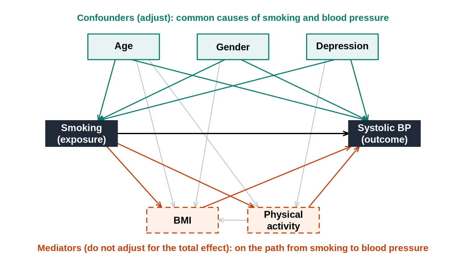
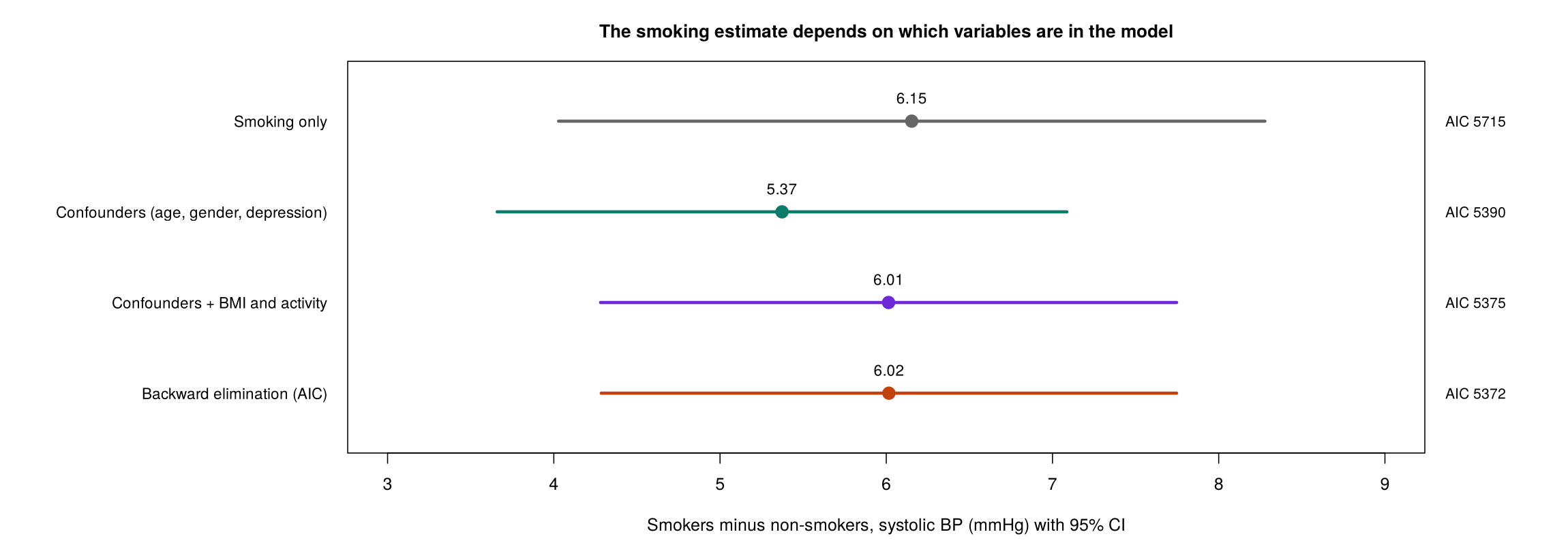
This section describes how to decide which variables enter a regression model and how to compare models. It starts from the goal of the analysis, shows how a causal diagram chooses the variables for an explanatory question, explains how many predictors the data can support, compares models with tests and information criteria, critiques automatic selection strategies, and shows how to test and interpret an interaction. It uses the PHAA survey with systolic blood pressure as the outcome and smoking as the exposure of interest, and every comparison uses the 748 participants with complete data for twelve candidate variables.
Before any variables are chosen, the analyst has to decide what the model is for, because the two common goals lead to different models. A model built to explain estimates the effect of an exposure on an outcome. Its variables are chosen to remove confounding, and its coefficients are interpreted, so the question is whether the coefficient for the exposure is free of bias. A model built to predict forecasts the outcome for new people. Its variables are chosen for accuracy, and its individual coefficients matter less, so the question is how close its predictions come to what actually happens. For example, BMI is left out of a model that estimates the total effect of smoking on blood pressure, because it lies on the path from smoking to blood pressure, but it could be kept in a model whose only aim is to predict blood pressure accurately, because it improves those predictions.
Most epidemiological questions, such as how much smoking raises blood pressure, are explanatory. Wording such as “the effect of” or “because of” points to explanation, while “predict”, “forecast” or “identify who is at risk” points to prediction. Click each of the three cards below to compare the two goals and to see the principle of parsimony, which applies to both.
The goal sets the rules for everything that follows: for explanation, a confounder stays even when it is not significant, and for prediction, a variable earns its place by improving accuracy for new people. For an explanatory question, the choice of variables starts from a causal diagram.
For an explanatory question, the variables are chosen before the results are seen, from subject-matter knowledge expressed as a causal diagram (also called a directed acyclic graph, or DAG). Each arrow is an assumed causal effect. A confounder has arrows to both the exposure and the outcome and is included in the model. A mediator lies on a path from the exposure to the outcome and is left out when the total effect of the exposure is of interest, because adjusting for it removes the part of the effect that travels through it.
Two further roles complete the picture. A collider has arrows pointing into it from both the exposure and the outcome (exposure → collider ← outcome), such as attending a clinic that both smokers and people with high blood pressure are more likely to attend. A collider is never adjusted for, because conditioning on it opens a non-causal path between the exposure and the outcome and can create a spurious association (collider or selection bias). By this we mean that restricting or adjusting for the collider builds a link that does not exist in the population. For example, among clinic attenders, a non-smoker must usually have some other reason to be there, such as high blood pressure, whereas a smoker may be there because of smoking alone. Within the clinic, smoking and high blood pressure can therefore appear negatively associated even if smoking had no effect on blood pressure at all. A moderator (effect modifier) is drawn with an arrow that points at the arrow from the exposure to the outcome, which means that it changes the strength of the effect. A moderator is not needed to remove confounding; it enters the model through an interaction term with the exposure, together with its own main effect, or the effect is reported separately in each of its groups, as 7.6 describes. Omitting a confounder biases the coefficient of the exposure through the open back-door path, and ignoring a moderator reports a single averaged effect that may describe neither group well.
Figure 3.10 shows the causal diagram for the effect of smoking on systolic blood pressure that this section uses.
Click each of the three cards below to see how the diagram separates the total effect of smoking from its direct effect, and why confounders and intervening variables are treated differently.
In the PHAA example, the confounder model therefore estimates the total effect of smoking, 5.37 mmHg, and adding the two mediators changes the question being answered rather than removing bias. Choosing variables is one step in a longer process: expand the four panels below for the six steps of model building, from specifying the largest model worth considering to presenting the result.
Identify the outcome variable and determine whether it needs transformation (e.g., natural log). Then identify the full set of predictors to consider. The maximum model includes all possible predictors of interest. While a large model prevents overlooking important predictors, adding too many increases the risks of collinearity and spurious associations. Key sub-steps include: drawing a causal diagram, potentially reducing predictors, considering missing values, evaluating effects of continuous predictors, and deciding on interaction terms. Section 2 describes how to decide whether the outcome needs a transformation.
Decide how you will determine which variables to retain. Criteria can be non-statistical (e.g., is it a primary predictor of interest? Is it a known confounder?) or statistical (e.g., partial F-tests, likelihood-ratio tests, information criteria like AIC or BIC). Both types of criteria should be considered together.
Choose how to apply the criteria. Options include: examining all possible subsets, forward selection (adding variables one at a time), backward elimination (starting with all variables and removing), or stepwise procedures (combining forward and backward). The strategy determines the order in which variables are evaluated. For a causal question these strategies are not used to choose confounders; 7.5 explains why.
Step 4: Conduct the analyses using your chosen strategy and criteria. Step 5: Evaluate the reliability of the chosen model using diagnostics and sensitivity analyses. Step 6: Present the results in a meaningful way, ensuring they are interpretable to your audience and that the model-building process is transparent. The end of this section lists what a report of the final model includes.
Step 1 warns that a maximum model with too many predictors carries risks, and the next subsection describes how many predictors the data can support.
Every estimated coefficient uses up information. By this we mean that a dataset contains only a fixed amount of evidence, and each coefficient the model estimates draws on that same pool, so the more coefficients there are, the less evidence supports each one. A common guide asks for at least 10 to 20 observations per coefficient in a linear model and at least 10 events per coefficient in a logistic model. A categorical predictor with k categories uses k − 1 coefficients. When a model has too many terms for its data, it starts to fit the random noise of its sample, which is called overfitting. Every sample contains chance patterns that would not appear in another sample from the same population, and a model with many terms has enough flexibility to follow those patterns as if they were real. As a result, its R² looks excellent, but its predictions for new people are poor, because the chance patterns it learned are not present in their data.
To check a proposed model, compare the number of observations, or of events for a logistic model, with the number of coefficients other than the intercept. The logistic model of Section 3 has 21 events per coefficient, comfortably above the guide, whereas the survey’s hypertension variable, with only 23 cases, could support only about two predictors. If the data cannot support a model, it is simplified on subject-matter grounds rather than by keeping only the terms that happen to be significant.
Interactive 3.4 shows overfitting at work. It fits curves of increasing flexibility (polynomial degree) to a small sample and tests them on new data from the same population. Slide the degree upwards and watch the fit to the sample keep improving while the error on the new data falls only up to a point and then rises; the best model for new data is the one at the bottom of that U shape.
Fit polynomials of increasing degree to a small training sample, then evaluate on a fresh hold-out sample drawn from the same true relationship. In-sample R², the fit to the training data, always rises as the curve becomes more flexible. Out-of-sample error, the error on the fresh hold-out points, first falls and then rises, forming a U shape. The degree at the bottom of the U gives the best predictions for new data.
A model that fits its sample well can still predict new data poorly, so competing models are compared with criteria that take their complexity into account, which the next subsection describes.
Models are compared only when they are fitted to the same observations. This matters because R quietly drops any person with a missing value on a variable in the model, so adding a predictor can also remove people. If the two models then differ in their fit, it is impossible to tell whether the difference comes from the new predictor or from the change in who was analysed. Because different predictors have different missing values, the safest approach is to create one complete-case data set for all candidate variables first, as the R activity does with na.omit().
Two models are nested when one model’s predictors are a subset of the other’s. By this we mean that the smaller model can be obtained from the larger one simply by deleting terms, as a model with age and smoking is nested within a model with age, smoking and BMI. Nested linear models are compared with a partial F-test, anova(m_small, m_large), and nested logistic models with a likelihood ratio test, anova(..., test = "Chisq"). In both cases a small p-value says that the extra terms explain enough additional variation to be worth the degrees of freedom they cost.
Not every pair of models is nested, however. A model with BMI and a model with physical activity in its place cannot be compared with these tests, because neither contains the other. Any models fitted to the same outcome and the same people, nested or not, can be compared with AIC and BIC instead. These information criteria trade fit against complexity: each one rewards a model for fitting the data closely and then adds a penalty for every parameter it estimates, so a larger model wins only if its better fit outweighs its extra cost. Lower values are better, and only the difference between two models carries information. The two criteria differ in the size of the penalty. BIC charges more for each extra term, so it tends to favour smaller models. Open each of the four tabs below to compare the criteria in more detail: the non-statistical reasons for keeping a variable, the tests for nested models, the information criteria with Equation 3.4, and adjusted R² and Mallows’ Cp with Equation 3.5.
Variables should be retained in the model if they:
A fourth, data-based check is often listed with these: a variable is kept if removing it changes the coefficient of interest substantially, often by more than 10% (the change-in-estimate criterion). This check uses the data, so it is a statistical criterion, and it cannot tell a confounder from a mediator, because removing a mediator also changes the coefficient of the exposure. It is therefore applied only to variables that the causal diagram already identifies as possible confounders, as a way of deciding whether a weak confounder can be dropped to gain precision.
Models where one model’s predictors are a subset of another’s are called nested models. Tests for nested models include:
For a categorical variable entered as several indicator terms, the overall significance of all its indicators is tested together in one test. The indicators together represent one variable, and the p-value of each separate indicator depends on which category was chosen as the reference.
In plain terms, each of these tests asks the same question: do the extra terms in the larger model explain enough additional variation to be worth the degrees of freedom they cost? A small p-value says yes.
For non-nested models, information criteria are used. Equation 3.4 gives the general formula:
Where s is the number of parameters, lnL is the log-likelihood, and a is a penalty constant. For AIC, a = 2 (Akaike, 1974). For BIC, a = ln(n) (Schwarz, 1978). Smaller values indicate a better model. Because ln(n) is larger than 2 whenever n is 8 or more, BIC charges more than AIC for each extra parameter and so tends to favour more parsimonious models, that is, models with fewer terms.
Reading the numbers. An AIC or BIC value means nothing on its own; a single value such as 1,240 is neither good nor bad. Only the difference between models carries information, and the comparison is valid only when the models are fit to the same outcome, measured the same way, on the same set of observations. That last condition catches beginners: you cannot compare the AIC of a model for Y against one for log(Y), and quietly dropping rows with missing values changes the sample, which makes the criteria incomparable.
Guidelines for interpreting BIC differences between models:
For AIC, a widely used rule of thumb reads the difference between each model and the model with the lowest AIC: a difference of 2 or less means the model still has substantial support, a difference of 4 to 7 means considerably less support, and a difference of more than 10 means essentially none (Burnham & Anderson, 2004).
For the PHAA example in this section, the model with BMI and physical activity has an AIC 15.0 lower (5374.7 against 5389.7) and a BIC 5.8 lower (5416.3 against 5422.1) than the model without them. Both criteria therefore favour the larger model, AIC strongly and BIC positively, in line with the partial F-test (F = 9.54, p < 0.001). R counts the error variance as one of the parameters, so a linear model with six coefficients has s = 7, which AIC() prints as df.
Adjusted R² is R² with a deduction for each predictor in the model, so it rises when a new predictor improves the fit by more than a predictor of pure noise would be expected to, and falls otherwise. The model with the highest adjusted R² is preferred. Mallows’ Cp, given in Equation 3.5, measures the same balance between fit and complexity, and lower values are better.
Here the sum of squares is taken over the candidate model; p is the number of parameters in the candidate model, counting the intercept, so a model with three predictors has p = 4; σ² is the mean squared error of the full model containing every candidate predictor; and n is the sample size. For the full model itself, Cp equals p by construction. Mallows’ Cp is closely related to AIC: when the error variance is treated as known and taken from the full model, the two differ only by a constant and rank candidate models in the same order. The decision rule used in this course is to prefer the candidate model with the lowest Cp.
Worked Example 3.9 applies these criteria to two nested models for systolic blood pressure, the larger of which adds BMI and physical activity; check whether the test and the two information criteria agree.
The smaller model contains age, gender, smoking and depression; the larger model adds BMI and physical activity. The partial F-test from anova(m_small, m_large) gives F = 9.54 on 2 and 740 degrees of freedom (p = 8.1 × 10⁻⁵), adjusted R² rises from 0.382 to 0.396, AIC falls by 15.0 (from 5389.7 to 5374.7) and BIC falls by 5.8 (from 5422.1 to 5416.3). Every statistical criterion favours the larger model. Worked Example 3.10 shows why that does not settle which model answers the question about smoking.
Fit statistics compare models that were specified in advance. The next subsection turns to strategies that select variables automatically, and to what happens when they meet an explanatory question.
When many candidate variables are available, selection strategies apply a criterion such as AIC or a p-value threshold automatically. Backward elimination starts with every candidate and removes terms one at a time, forward selection starts with none and adds them, and stepwise selection does both, checking at each step whether an earlier choice should be reversed. Click each of the three cards below for more on all possible subsets, forward selection with its stepwise variant, and backward elimination.
In R, step(m_full, direction = "backward") performs backward elimination by AIC. Starting from all 11 candidate predictors (age, gender, smoking, depression, BMI, physical activity, anxiety, social support, discrimination, education and region), it keeps age, smoking, depression, BMI and physical activity. AIC-based elimination keeps any term whose removal would raise AIC, which corresponds roughly to keeping terms with a p-value below about 0.16, so physical activity (p = 0.14 in the full model) is retained. Gender is dropped, although the causal diagram in Figure 3.10 treats it as a confounder.
Automatic strategies choose variables by how well they fit the sample, so they cannot distinguish a confounder from a mediator, they can drop a confounder that adds little to the fit, and they can keep a mediator that predicts the outcome well. The p-values and confidence intervals of the selected model are also too optimistic, because the same data were used to choose the model and to test it. For an explanatory question, the causal diagram decides which variables are included; automatic selection is better suited to prediction or to exploring a large set of candidates.
Worked Example 3.10 compares the smoking estimate from four models fitted to the same 748 people, including the model chosen by backward elimination. Figure 3.11 shows the four estimates, and Table 3.11 lists them with their confidence intervals, their AIC and what each model estimates; compare the lowest-AIC model with the confounder model from the causal diagram.
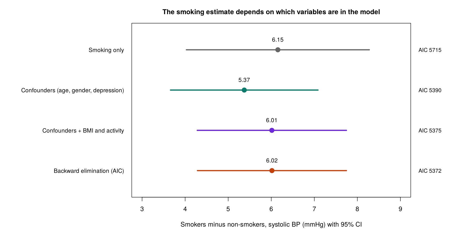
Table 3.11. The smoking estimate, its 95% confidence interval and the AIC from each of the four models, with what each model estimates.
| Model | Smoking estimate (mmHg) | 95% CI | AIC | What it estimates |
|---|---|---|---|---|
| Smoking only | 6.15 | 4.03 to 8.28 | 5714.9 | The crude difference, affected by any confounding. |
| Confounders from the causal diagram (age, gender, depression) | 5.37 | 3.66 to 7.09 | 5389.7 | The total effect of smoking, if the diagram is correct. |
| Confounders + BMI and physical activity | 6.01 | 4.28 to 7.75 | 5374.7 | The effect of smoking other than through BMI and activity. |
| Backward elimination by AIC | 6.02 | 4.29 to 7.75 | 5371.7 | A mixture chosen by fit, which drops gender and keeps the mediators. |
The models with the mediators have the lower AIC, mainly because BMI predicts blood pressure well. In these data, smokers have a lower average BMI (19.3 against 21.1 among these 748 people), so part of the effect of smoking on blood pressure is counteracted through BMI, and adjusting for BMI removes that counteracting path and raises the smoking estimate. For the question "how much higher is blood pressure because of smoking?", the confounder model, with an estimate of 5.37 mmHg, is the appropriate one. Fit statistics then help to choose among models that answer the same question, for example a straight-line term for age against a curved one.
The model with the best fit is not automatically the model that answers an explanatory question. The last subsection turns to interactions, where the effect of one predictor depends on another.
An interaction (effect modification) is present when the effect of one predictor depends on the value of another. By this we mean that there is no single answer to a question such as “how much higher is blood pressure in smokers?”, because the answer differs from one group of people to another. For example, if smoking raised blood pressure by 8 mmHg in younger adults but by only 3 mmHg in older adults, the effect of smoking would depend on age. A model without an interaction cannot represent this, because it forces the smoking difference to be the same at every age. Adding an interaction term relaxes that restriction by allowing the slope for one predictor to change with the value of the other. In R, age * smoker adds age, smoking and their product age:smoker. Comparing lm(systolic_bp ~ age * smoker + gender + dep_score) with the model without the product gives F = 1.08 on 1 and 741 df (p = 0.30), so there is no evidence that the effect of smoking changes with age, and the simpler model is kept. An interaction term is always fitted with both of its main effects, and the interactions to test are best chosen in advance. Expand the five panels below for common strategies for choosing which interactions to test, of which the theory-driven ones are preferred.
This is feasible only when the total number of predictors is small (e.g., ≤ 8). You create and test every possible pair of interaction terms.
After building the final main-effects model, create interactions among all predictors that are statistically significant. This reduces the number of interactions to evaluate but may miss interactions with non-significant main effects.
Create interactions among all predictors that have a significant unconditional association with the outcome. This casts a wider net than Strategy 2.
Only create interactions among pairs of variables you suspect (based on evidence from the literature or biological reasoning) might interact. This usually focuses on interactions involving the primary predictor(s) of interest and important confounders.
Only create interactions that involve the exposure variable (primary predictor of interest). This is the most conservative approach but may miss important interactions among covariates.
A test says whether an interaction is present; Worked Example 3.11 shows how the coefficients of a model with an interaction are read, and why centring the continuous partner makes the main effect readable.
With an interaction, the model for blood pressure contains age, smoking and their product. Written for one continuous predictor X1 (age) and a 0/1 indicator X2 (smoking), it is Y = β0 + β1X1 + β2X2 + β3X1X2 + the other terms. The slope of X1 is then β1 + β3X2, so it differs between the two groups. By this we mean that among non-smokers (X2 = 0) the slope for age is β1, while among smokers (X2 = 1) it is β1 + β3, so β3 is the difference between the two slopes. In the same way, each main effect describes its own variable’s effect at the point where its partner equals 0: β1 is the effect of age among non-smokers, and β2 is the effect of smoking at age 0. The main effects therefore no longer have a single overall meaning, and each must be read at a stated value of its partner.
In lm(systolic_bp ~ age * smoker + gender + dep_score), the coefficient for smokerYes is 8.24 mmHg, but it is the difference between smokers and non-smokers at age 0, which lies outside the data. Centring age at 45 years, close to its mean, makes the main effect readable without changing the fit:
smokerYes (5.39 mmHg): at age 45, smokers have a mean systolic blood pressure 5.39 mmHg higher than non-smokers of the same gender and depression score. Because the model contains the interaction, this is the gap at age 45 only.age_c (0.46 mmHg per year): the slope of blood pressure on age among non-smokers, the reference category of the partner variable.age_c:smokerYes (−0.063 mmHg per year): the slope of age is 0.063 mmHg per year smaller for smokers than for non-smokers, so the slope among smokers, which the code you add in question 3 of Activity 3.4 prints, is about 0.40 mmHg per year. Equivalently, the gap between smokers and non-smokers narrows slightly as age rises. Its p-value of 0.30 gives no evidence that the gap really changes with age, so the main-effects model is kept.Had the interaction been clearly significant, the substantive conclusion would be stated in one sentence about both groups, for example "smoking is associated with a larger rise in blood pressure among younger adults than among older adults", and the effect of smoking would be reported at chosen ages rather than as one number.
Once the product term is in a model, each main effect must be read at a stated value of its partner, and the interaction itself is described for both groups.
This part is background for writing up an analysis rather than an exam objective. A report of a regression model states the goal of the analysis and how the variables were chosen (with the causal diagram, if one was used), the number of people analysed out of the number available, each estimate on its own scale (a difference in means for a linear model, an odds ratio for a logistic model) with its 95% confidence interval, the checks that were carried out and their results, and any sensitivity analyses, such as the same model with an alternative set of variables.
The narrated walkthrough below compares nested models and demonstrates the selection strategies of 7.5 on a second dataset, as optional practice before the activity.
This walkthrough compares nested regression models with F-tests, adjusted R-squared, the AIC and the BIC, keeping the same people in every model, and then shows backward elimination and forward selection with their limitations.
Open the Comparing Models and Selecting Variables in R walkthroughActivity 3.4 practises 7.2 to 7.6. Run along to create one complete-case data set for the twelve candidate variables, compare two nested models, test gender as a whole, run backward elimination and test an interaction between age and smoking, answering three questions in the style of the midterm along the way.
Text version of the activity: the code of the run-along script, its console output and notes on reading it.
phaa <- read.csv("https://heal-learn.ca/r-activities/data/phaa_survey_clean.csv")   # course data, read from the website
phaa$smoker <- factor(phaa$smoker, levels = c("No", "Yes"))   # "No" = reference
phaa$gender <- factor(phaa$gender, levels = c("Man", "Woman", "Non-binary"))
vars <- c("systolic_bp", "age", "gender", "smoker", "dep_score", "bmi", "phys_act_min",
          "anx_score", "social_support_score", "discrimination_score", "education", "region")
build <- na.omit(phaa[, vars])   # the same people for every model compared
nrow(build)Every model below uses these 748 people, so their F-tests, AIC and BIC values can be compared.
m_small <- lm(systolic_bp ~ age + gender + smoker + dep_score, data = build)
m_large <- lm(systolic_bp ~ age + gender + smoker + dep_score + bmi + phys_act_min, data = build)
anova(m_small, m_large)          # partial F-test for the two added terms
round(c(adjR2_small = summary(m_small)$adj.r.squared,
        adjR2_large = summary(m_large)$adj.r.squared), 3)
AIC(m_small, m_large); AIC(m_large) - AIC(m_small)   # lower is better
BIC(m_small, m_large); BIC(m_large) - BIC(m_small) # a larger penalty per termround(summary(m_small)$coefficients, 4)
m_nogen <- lm(systolic_bp ~ age + smoker + dep_score, data = build)
anova(m_nogen, m_small) # both gender indicators tested togetherm_full <- lm(systolic_bp ~ ., data = build) # every other column of build
m_back <- step(m_full, direction = "backward", trace = 0)
formula(m_back)
round(sapply(list(confounders = m_small, backward = m_back),
function(m) coef(m)[["smokerYes"]]), 2) # smoking estimatessystolic_bp ~ . means "systolic blood pressure on every other column of build". trace = 0 hides the step-by-step printout; trace = 1 shows each step.
m_int <- lm(systolic_bp ~ age * smoker + gender + dep_score, data = build)
anova(m_small, m_int)            # tests the product term age:smoker
round(summary(m_int)$coefficients, 4)The interaction is tested by comparing two models that differ only by the product term age:smoker and are fitted to the same 748 people. In the model with the product, smokerYes is the gap between smokers and non-smokers at age 0.
Answer each question from your own output, as on the midterm: make the decision, give each reason with the number that supports it, and keep the theory and the statistics apart.
1. Report the partial F-test comparing m_small and m_large with its degrees of freedom, the two adjusted R² values and the AIC and BIC differences that lines 21 and 22 print. Which model does each criterion favour, and why can these values be compared?
m_large (line 21 prints −15.04; 5374.7 against 5389.7), more than 10, and BIC is 5.8 lower (line 22 prints −5.80; 5416.3 against 5422.1), positive evidence on the BIC scale; BIC charges more for each extra term, so its difference is smaller. Every criterion favours m_large, and the values can be compared because both models are fitted to the same outcome and the same 748 people. These criteria measure fit only; whether BMI and physical activity belong in a model for the effect of smoking is decided by the causal diagram.2. A colleague says: “Backward elimination dropped gender, and neither gender indicator in m_small is significant, so we should remove gender and report the smoking estimate of 6.02 mmHg from m_back.” Based on these results and the causal diagram in Figure 3.10, do you agree? Explain why or why not.
confint(m_small)).3. Run your own code: at the end of your script, type build$age_c <- build$age - 45, m_int_c <- lm(systolic_bp ~ age_c * smoker + gender + dep_score, data = build) round(summary(m_int_c)$coefficients, 4) and round(coef(m_int_c)[["age_c"]] + coef(m_int_c)[["age_c:smokerYes"]], 4) on four lines and run them (the last line gives the slope of age for smokers). Interpret the coefficient on smokerYes and the interaction coefficient age_c:smokerYes, attaching units and naming the comparison each makes, and describe in one sentence what the interaction means substantively.
smokerYes (5.39 mmHg): at age 45, smokers have a mean systolic blood pressure 5.39 mmHg higher than non-smokers of the same gender and depression score. Because the model contains the interaction, this is the gap at age 45 only, not a single overall effect of smoking; in m_int the same coefficient, 8.24 mmHg, was the gap at age 0, outside the data, and centring changed only where the gap is read, not the fit. age_c:smokerYes (−0.063 mmHg per year): the slope of blood pressure on age is 0.063 mmHg per year smaller for smokers than for non-smokers: the age_c row gives the slope for non-smokers, 0.46 mmHg per year, and the last line of your code prints the slope for smokers, 0.40, so the smoking gap narrows slightly as age rises. The test of the product term, which compares two models that differ only by age:smoker and are fitted to the same 748 people, gives F = 1.08 on 1 and 741 df (p = 0.30), so there is no evidence that the gap changes with age. Substantively, the difference in blood pressure between smokers and non-smokers is about the same at every age in these data, so the model without the interaction is kept and the effect of smoking is reported as one number, 5.37 mmHg.The activity reproduces the comparisons in Worked Examples 3.9 to 3.11. This section has shown how the goal of a model, a causal diagram and comparisons between models guide the choice of variables, and what a report of the final model includes. The knowledge check that follows reviews these points.
sum(cc$y01) / (length(coef(logit)) - 1), which prints 21 for the logistic model of Section 3, comfortably above the guide of about 10. The survey's hypertension variable, with only 23 cases, could support only about two predictors. If the data cannot support the model, simplify it on subject-matter grounds rather than keeping only the terms that happen to be significant.anova(m_small, m_large)) or a likelihood ratio test for a logistic model (anova(..., test = "Chisq")); a small p-value says the extra terms improve the fit. For any models fitted to the same outcome and the same people, nested or not, AIC and BIC trade fit against complexity: lower is better, only the difference between models carries information, and BIC charges more for each extra term, so it tends to favour smaller models (in Worked Example 3.9, adding BMI and physical activity lowered AIC by 15.0 and BIC by 5.8). The trap most students fall into is comparing models fitted to different people, which happens silently when the added variables have missing values, so create one complete-case data set with na.omit() for all candidate variables first, and never compare the AIC of a model for Y with one for log(Y). Remember, too, that the best-fitting model is not automatically the right one for an explanatory question.step(m_full, direction = "backward") eliminates by AIC. All three choose variables by how well they fit the sample, so they cannot tell a confounder from a mediator: in the PHAA data, backward elimination dropped gender, which the causal diagram treats as a confounder, and kept BMI and physical activity, which are mediators of smoking. The p-values and confidence intervals of the selected model are also too optimistic, because the same data were used to choose the model and to test it. To critique an automatically selected model, check each variable it kept or dropped against the causal diagram and say what question the resulting estimate really answers (here about 6.0 mmHg, a mixture, instead of the total effect of 5.37 mmHg). Automatic selection is better suited to prediction or to exploring a large set of candidates.age * smoker fits both main effects and their product, age:smoker, and the interaction is tested by comparing the models with and without the product term on the same people (here F = 1.08, p = 0.30, so the simpler model is kept). Once the product is in the model, each main effect is the effect of its variable when its partner equals 0 (or is at its reference category), and the product coefficient is the difference in slopes between the groups, so the slope of X1 is β1 + β3X2. That is why the uncentred smokerYes coefficient of 8.24 mmHg is the gap between smokers and non-smokers at age 0, whereas centring age at 45 gives 5.39 mmHg, the gap at age 45. When you interpret an interaction model, say where each main effect applies ("at age 45", "among non-smokers"), give the slope in each group (R gives the slope among smokers in one line, coef(m_int_c)["age_c"] + coef(m_int_c)["age_c:smokerYes"], about 0.40 mmHg per year), keep both main effects alongside the product, and finish with one sentence about what the interaction means for both groups.1. Two analysts use the same hospital data. Analyst A wants to estimate the effect of a new discharge programme on readmission; Analyst B wants a tool that predicts which patients will be readmitted. Which approach to choosing variables fits each goal?
2. A causal diagram for the effect of regular physical activity (A) on a depression score (Y) shows: age, with arrows to both A and Y; sleep quality, on the path A → sleep → Y; use of the campus wellness centre, with arrows into it from both A and Y; and gender, drawn with an arrow that points at the A → Y arrow. The total effect of A is wanted. Which model follows the diagram?
A * gender fits together with both main effects. Option b is the tempting error, since it treats sleep correctly, but adding the collider introduces collider bias; option d adjusts away the part of the effect that passes through sleep and averages the effect over the gender groups. (Section 4, 7.2 Choosing Variables From a Causal Diagram; Objective 7.2)3. A logistic regression for a rare surgical complication is planned in 500 patients. The candidate predictors are age, sex, a four-category region and five other continuous measurements, and R gives the counts below for the data and for a trial fit of the full model. Can the data support all of these predictors?
4. Two linear models for systolic blood pressure are fitted to the same 900 people. Model 1 contains age and sex; Model 2 adds a diet score and minutes of activity. anova(model1, model2) gives F = 6.1 on 2 and 895 df (p = 0.002), and R prints the information criteria below. Which reading is correct?
5. To estimate the total effect of alcohol use on systolic blood pressure, a colleague ran backward elimination by AIC. It dropped income, which the causal diagram treats as a confounder, and kept body weight, which the diagram treats as a mediator. The colleague reports the alcohol coefficient and its p-value from the selected model. What is the main problem?
6. A model for systolic blood pressure is fitted with lm(sbp ~ salt_c * diabetes + age), where salt_c is daily salt intake in grams minus 8, and diabetes is Yes or No, with No as the reference category. The estimates, in mmHg, are salt_c 0.8, diabetesYes 4.0 and salt_c:diabetesYes 0.6 (p = 0.01), and R gives the line below. Which interpretation is correct?
7. A cohort study asks whether sugar-sweetened beverages (ssb, servings per day) raise fasting blood glucose (mmol/L) in 820 adults. In the causal diagram, age, household income and physical activity each affect both SSB intake and glucose; body mass index (bmi) lies on the path from SSB intake to glucose; and a recent diabetes screening visit (visit) is more likely both for heavy SSB drinkers and for people with high glucose. The four models below were fitted to the same 820 people, and a colleague proposes reporting Model D because it has the lowest AIC. Which response is best?
| Model | SSB estimate per daily serving (95% CI) | AIC |
|---|---|---|
A: ssb only | 0.195 (0.145 to 0.245) | 1682.8 |
B: ssb + age + income + activity | 0.187 (0.137 to 0.237) | 1626.2 |
C: Model B + bmi | 0.123 (0.074 to 0.172) | 1536.0 |
D: chosen by step(), which kept ssb, age, income, bmi and visit | 0.084 (0.036 to 0.133) | 1477.6 |
bmi is a mediator, so adjusting for it (Models C and D) removes the part of the effect that travels through body weight, and visit is a collider, so adjusting for it (Model D) opens a non-causal path and can create a spurious association. Option a is the tempting error: bmi and visit predict glucose well, which lowers the AIC, but fit statistics do not encode the causal question, and Model D was also chosen automatically and dropped activity, a confounder. Option b ignores the difference between confounders, mediators and colliders, and option d leaves the confounding by age, income and activity in place. (Section 4, 7.2 Choosing Variables From a Causal Diagram, 7.5 Variable Selection Strategies and Their Limits, the callout "Limits of Automatic Selection" and Worked Example 3.10; Objectives 7.2 and 7.5)This lesson moved from comparing two variables to building and comparing regression models. Section 1 matched each pair of variable types to a two-variable test, listed the rank-based and exact alternatives used when an outcome is skewed or ordinal or when counts are small, applied the correlation coefficient, the t-test, ANOVA and the chi-square test to the PHAA survey, and showed with physical activity and blood pressure that a two-variable comparison can be distorted by confounding: the difference of 2.8 mmHg per 100 minutes of activity fell to 0.9 mmHg once age was taken into account. It then introduced the regression line, least squares and the multivariable model, in which each coefficient is adjusted for the other predictors, and showed that the t-test is a regression with one binary predictor.
Section 2 fitted a linear regression for systolic blood pressure with five predictors, in which smokers averaged 6.1 mmHg higher than comparable non-smokers and the model explained 41% of the variation. The model passed each check: the four diagnostic plots, a squared age term, the Breusch-Pagan and Shapiro-Wilk tests, Cook's distance and variance inflation factors. The section also described the standard responses when a check fails, such as a squared term, a log transformation or sandwich standard errors. Section 3 modelled elevated blood pressure with logistic regression, in which smokers had 5.8 times the odds of comparable non-smokers, explained odds, log odds and predicted probabilities, and checked the model for events per coefficient, linearity on the log-odds scale, calibration (Hosmer-Lemeshow p = 0.59) and discrimination (AUC = 0.86). Section 4 showed that the choice of variables starts from the goal of the analysis and, for an explanatory question, from a causal diagram; that models are compared on the same people with F-tests, likelihood ratio tests, AIC and BIC; and that the best-fitting model, which included two mediators of smoking, was not the right model for estimating the total effect of smoking.
lm() fit (t = estimate ÷ SE, its p-value and the 95% CI of about the estimate ± 1.96 SE) and the statistics for the whole model: R², adjusted R², the residual standard error, the F-test and the analysis of variance table. Remember that the Adjusted R-squared printed by summary(), which is 1 − MSE ÷ MST, is the answer whenever a question asks for the variance explained after penalising for unnecessary predictors.lm() is the wrong tool for a 0/1 outcome, and interpret a glm(..., family = binomial) model through its exponentiated coefficients (adjusted odds ratios) and its predicted probabilities. Remember that the odds ratio for a change of more than one unit multiplies the coefficient by Δx before exponentiating, as exp(10 * coef(fit)["age"]) does in R, and that an odds ratio exaggerates the risk ratio when the outcome is common, so describe it as a ratio of odds, not of risks.The final assessment covers all four sections. All 16 questions must be answered correctly (100%) to finish the lesson.
1. A pilot study gives drug A to 12 patients and drug B to 12 patients. One patient on drug A and 5 on drug B have an adverse reaction, and R prints the expected counts below. Which test should compare the proportions with a reaction?
2. A linear model for a sleep-quality score (points), saved as fit, includes screen time entered as ln(minutes + 1), with a coefficient of −0.90, holding age constant. The analyst compares a person with 99 minutes and a person with 9 minutes of screen time a day, at the same age, with the line below. What does the result mean?
3. A linear model for HbA1c (%) is fitted with lm(hba1c ~ age_c + sex + bmi_c), where age_c is age minus 50, bmi_c is BMI minus 25, and sex has Man as the reference category. The intercept is 5.9. What does the intercept represent?
4. The bottom of the summary() output for a linear model of a mobility score (points) with five predictors, fitted to 600 people, reads: "Residual standard error: 6.4 on 594 degrees of freedom; Multiple R-squared: 0.262, Adjusted R-squared: 0.256; F-statistic: 42.2 on 5 and 594 DF, p-value: < 2.2e-16". Which statement reads it correctly?
5. In a linear model for a depression score (points), the coefficient comparing rural with urban residents is 1.2 (95% CI −0.4 to 2.8, p = 0.14), holding age and income constant. Which conclusion is correct?
6. A linear model for systolic blood pressure has a Residuals vs Fitted plot whose red smoother is U-shaped, a Q-Q plot with the points on the diagonal, a flat Scale-Location line and no point beyond a Cook's distance contour; crPlots() shows a curved line for BMI only. Which assumption is in doubt, and what is the first response?
anova(old, new); centring BMI before squaring keeps the two terms from being strongly collinear. Option c is tempting because the Residuals vs Fitted panel is also used to check equal variance, but unequal variance shows as a funnel and a rising Scale-Location line, not as a U-shaped curve with a flat Scale-Location line. Independence is judged from the study design rather than from these plots. (Section 2, 4.1.1 Reading the Four Diagnostic Panels, Table 3.5, Figure 3.4, the 4.1.6 accordion on component-plus-residual plots, 4.3 Responding When a Check Fails and Table 3.6; Objectives 4.1 and 4.3)7. A linear model includes both BMI and waist circumference, two measures of body size, and R prints the values below for waist circumference. What do they mean?
8. A logistic model for a positive screening test includes smoking (smoker = 1 for smokers, 0 for non-smokers) and other predictors. For a smoker at the average values of the other predictors, R prints the value below. What does it mean?
type = "response" asks for: with this argument, predict() returns predicted probabilities, so 0.27 means that about 27 in every 100 smokers at these values of the other predictors are expected to test positive (R applies p = 1 ÷ (1 + e−(log odds)), Eq 3.2, for you). Options a and b are the tempting errors: the log odds, the odds and the probability are three scales for the same prediction, and here the log odds are −1.0 and the odds about 0.37, so neither is the number printed. Option c confuses a prediction for one kind of person with a comparison between two groups. (Section 3, 5.2 Probability, Odds and Log Odds, Eq 3.2, 5.4 Predicted Probabilities, and Why an Odds Ratio Is Not a Risk Ratio, and Worked Example 3.7; Objective 5.4)9. In a logistic model for low back pain, which affects about 35% of the sample, the adjusted odds ratio for physical inactivity is 1.8 (95% CI 1.2 to 2.7), holding age, sex and occupation constant. Which interpretation is correct?
10. A colleague fits lm() to a 0/1 outcome in 3,000 people and argues that the model is acceptable: its coefficients are easy to read as differences in probability, and with 3,000 people a failed Shapiro-Wilk test does not matter. The output also shows 85 fitted values below 0 and a Breusch-Pagan test with p < 0.001. Which reply is best?
11. Region, with four categories, is added to a logistic model, and the two models, fitted to the same people, are compared as shown below. What does the result show?
anova() output: the residual deviance falls by 8.4 when region is added, on 3 degrees of freedom, with p = 0.04. A factor with four categories enters as three indicator variables, so the likelihood ratio test of region as a whole has 3 df, one for each term added, and its p-value shows that the three indicators together, that is, region as a whole, improve the fit. Option b is the tempting error: region is one variable, but it costs three coefficients, and the degrees of freedom count the terms added or removed, not the variables. Option c misreads the degrees of freedom as a count of significant comparisons, and option d confuses a drop in deviance with a share of variance. (Section 3, 6.1 Checking a Logistic Model: Events, Linearity and Tests, and Worked Example 3.8, and Section 4, 7.4 and the tab "Nested Models"; Objective 6.1)12. A logistic model that predicts hospital readmission has an area under the ROC curve of 0.88, but the Hosmer-Lemeshow test gives p = 0.003. Which interpretation is correct?
13. A study asks whether a stressful job (the exposure) affects a migraine score (the outcome). A colleague proposes adjusting for "visited a neurologist in the past year", which both a stressful job and frequent migraines make more likely. What is the likely consequence of adjusting for it?
14. Two linear models are fitted to the same outcome, but because of missing values one uses 790 people and the other 748. The second has the lower AIC. Can the AIC values be compared to choose between the models?
na.omit(), and to refit both models to those 748 people. Option b is the tempting error, because AIC can indeed compare models that are not nested, but only on the same rows; option c confuses the condition for F-tests and likelihood ratio tests (nesting) with the condition for AIC (the same data), and even nested models must use the same people. (Section 4, 7.4 Comparing Models and the tab "Information Criteria"; Objective 7.4)15. Researchers fit lm(fev ~ smoker * sex + age + height), where fev is a lung-function measure in litres and the reference categories are non-smoker and man. The estimates are smokerYes −0.10, sexWoman −0.40 and smokerYes:sexWoman −0.15, and the F-test comparing this model with the one without smoker:sex gives p = 0.002. R also gives the line below. How should the smoking result be reported?
16. A regional survey of 1,050 adults asks whether weekly hours of unpaid caregiving are associated with poor sleep (poor_sleep = 1 for the 181 people who usually sleep fewer than 6 hours a night). The team first fitted lpm <- lm(poor_sleep ~ care_hrs + age + gender + income + employment). A colleague notes that every fitted value lies between 0 and 1 and concludes that lm() is acceptable for this outcome. Based on the output below, which reply is best?
lm() are unreliable, and for any fitted value p̂ a residual can only be 1 − p̂ or −p̂, so the residuals cannot be normal. Option b is the tempting error, because a large sample helps with non-normal residuals but does nothing about the unequal variance. Option a ignores the two failed checks, and option d fails because the logarithm of 0 is undefined. (Section 3, 5.1 Why Linear Regression Does Not Suit a Binary Outcome, and Worked Example 3.6; Objective 5.1)✦ Before submitting: pass every section knowledge check (100%).