A Structured Approach to Data Analysis
Exploratory Data Analysis For Epidemiology
Learning objectives for this lesson:
- Explain why a structured, iterative and reproducible workflow, which starts with a causal diagram and runs every step from a script (program mode), gives more trustworthy results than going straight to a multivariable model.
- Identify the outcome, the exposure, and any confounders, mediators (intervening variables) and colliders in a causal diagram.
- Choose the adjustment set that follows from a causal diagram, and explain the consequence of omitting a confounder, adjusting for a mediator when the total effect is wanted, or adjusting for a collider.
- Identify coding faults in a raw data file (missing-value codes that could be real values, text in numeric fields, compound codes, and inconsistent formats or missing-value conventions) and state how each should be corrected according to best practice.
- Describe a system for managing data-collection sheets, data entry, files, variables and analyses that protects the original data and leaves an audit trail.
- Describe the scripted editing and verification checks made on each variable before analysis, and use their output to identify implausible values and unexpected categories.
- Choose how to process the outcome and predictor variables for the planned analysis, choose the unconditional analysis for each pair of variable types, and explain what these first analyses reveal before multivariable modelling.
This course was developed by Dr. Kiffer G. Card based on Dohoo, I. R., Martin, S. W., & Stryhn, H. (2012). Methods in Epidemiologic Research. VER Inc.
Glossary: Key Terms, People & Concepts
📚 Reference page, available throughout the lesson
This glossary collects the key concepts, people, and ideas you will meet in this lesson. Use it as a reference while you work through the material, or as a review before assessments. Type in the search box to filter entries.
Introduction & Data Collection
Overview
This course addresses how to analyse the data that epidemiological studies produce. It uses R to apply the main statistical methods of modern public-health analysis, including linear, logistic, multinomial, ordinal, and count regression; mixed models for clustered and longitudinal data; and causal-inference tools for observational data. None of these models is needed to follow this lesson. This first lesson sets the foundation: a disciplined workflow for taking raw data from collection through to analysis-ready files. This section explains why that workflow matters, shows how a causal diagram decides which variables belong in a model before any data are touched, and sets up the storage of the original data, on paper and in files.
Learning Objectives
- 1.1 Explain why a structured, iterative analytic workflow outperforms diving straight into modelling, and name its steps from the causal diagram to the multivariable model.
- 2.1 Sketch a causal diagram and identify the outcome, the exposure, and any confounders (forks), mediators or intervening variables (chains) and colliders in it.
- 3.1 Read the adjustment set from a causal diagram, and explain what goes wrong when a confounder is omitted, a mediator is adjusted for when the total effect is wanted, or a collider is adjusted for or selected on.
- 5.1 Set up a storage and tracking system for original data-collection sheets.
1.1 Why a Structured, Iterative Workflow
When starting the analysis of a complex dataset, it is very helpful to have a structured approach in mind. For most people, there is a strong tendency to jump straight into the sophisticated analysis that will provide the ultimate answer. This rarely works out, because the results will be wrong when important preliminary steps were skipped. A model fitted before the data are cleaned inherits every coding error in the file, and a model built without a causal diagram has no stated estimand (the effect being estimated) or adjustment set, so its results can look reasonable and still be wrong.
The structured approach has become especially important since the wider scientific community recognised a replication crisis in published research (Ioannidis, 2005; Open Science Collaboration, 2015) and called for a manifesto of reproducible practice (Munafò et al., 2017). The crisis concerns two ideas that are easily confused, and the distinction explains what the habits in this lesson are for.
Replication and Reproducibility
Replication means repeating a study with new participants and new data to see whether the original finding holds. Reproducibility means re-running the original analysis on the original data, with the original code, and obtaining the same numbers. The crisis was named for failed replications, which Ioannidis warned about in 2005 and which large projects documented in the 2010s. The habits taught in this lesson target reproducibility, because a result that cannot be reproduced from its own data and code cannot be checked, corrected, or built upon.
The workflow taught in this course follows a template whose steps are taken in order. The analyst first draws a causal diagram of the question, then cleans and verifies the data, then runs simple unconditional checks (one predictor at a time, with nothing else held constant), and only then fits the multivariable model. The order matters because each step depends on the one before it: the diagram decides which variables belong in the model, and the unconditional checks can be trusted only once the data have been verified. A plan that lets p-values choose the variables reverses this order, because the data, rather than the causal question, then decide what is adjusted for. The principle behind the template is stated below, together with three terms that recur throughout the course.
Key Principle: Analysis Is Iterative
Data analysis is an iterative process which often requires that you back up several steps as you gain more insight into your data, an idea Tukey developed when he distinguished exploratory from confirmatory work (Tukey, 1980). A structured template, while not the only approach, will be applicable in most situations and will serve to guide your initial efforts; tidy-data conventions (Wickham, 2014) make each iteration cheaper.
Three terms recur throughout the course. Exploratory analysis means getting to know the data by summarising and plotting it and looking for patterns, errors, and surprises; confirmatory analysis means formally testing a claim that was stated before the data were examined. Tidy data means a table in which each variable has its own column, each observation (for example, each participant) has its own row, and each cell holds a single value.
Iteration means that the template is a loop rather than a straight line. A problem found while verifying the data, or a surprising unconditional association, sends the analyst back to recode a variable or to reconsider the diagram, and backing up in this way is the normal pattern of an analysis rather than a sign of failure. The first step of the template, taken before any work with the data begins, is the causal diagram.
2.1 Sketching a Causal Diagram
Before you start any work with your data, it is essential to construct a plausible causal diagram of the problem you are about to investigate. The diagram identifies which variables are the important outcomes and predictors, which are potential confounders, and which might be intervening variables between the main predictors and the outcomes. A causal diagram is a drawing in which each variable is a box and each arrow states a belief that one variable causes another. By this we mean that the diagram is a written record of what the analyst assumes about how the variables are related, made before the data can influence those assumptions. Because every later decision about which variables to include in a model is read from these arrows, keep the diagram in mind throughout the entire data-analysis process. With large datasets it will not be possible to include every predictor as a separate box, and this can be handled by drawing blocks of variables in place of the individual variables. For example, age, sex and income might be drawn as a single box labelled “demographic characteristics”, with one arrow for the whole block, which keeps the diagram readable while still recording the role that the block plays.
The callout below recalls the kind of causal diagram used in this course and its three structures, each with the adjustment rule that goes with it; these rules are used in every later lesson, so commit them to memory.
Recall: DAGs and Their Three Structures
When we say “causal diagram” in 410, we mean a directed acyclic graph (DAG): nodes for variables, directed arrows for direct causal effects, no cycles. The three structural pieces you met in an earlier course still do all the work:
- Fork (X ← C → Y): C is a confounder. Adjust for it.
- Chain (X → M → Y): M is a mediator. Do not adjust if you want the total effect.
- Collider (X → Z ← Y): Do not adjust, and watch for it in selection.
The DAG fixes your estimand (what causal quantity you are estimating) and your adjustment set (what goes on the right-hand side of the regression) before you fit anything. In 410 we use it as the bridge from a research question to a regression model.
Worked Example 1.1 applies the three structures to the smoking cohort used in Activity 1.1, building the diagram in six steps from the research question to the adjustment set. Table 1.1 lists the steps and Figure 1.1 shows the finished diagram; as you read, watch how each variable’s role is decided by the direction of its arrows.
Worked Example 1.1: From a research question to a DAG and an adjustment set
The smoking cohort used in Activity 1.1 (cohort.csv) records whether each participant smokes and whether an event occurred during follow-up. Suppose the event is a cardiovascular (CVD) event, such as a heart attack or stroke. The six steps in Table 1.1 turn that study into a causal diagram.
Table 1.1. Six steps from the research question to the adjustment set for smoking and cardiovascular (CVD) events in the smoking cohort.
| Step | What the analyst does | Result for this example |
|---|---|---|
| 1. State the question | The question names the population, exposure, comparator, and outcome (PECO). | Among adults aged 20 to 79, does smoking, compared with not smoking, increase the risk of a CVD event during follow-up? |
| 2. Add common causes | The analyst lists variables that plausibly cause both the exposure and the outcome, using subject-matter knowledge and earlier studies. | Age and sex both influence whether a person smokes and their CVD risk, so each gets an arrow into smoking and an arrow into the CVD event. |
| 3. Add pathway variables | The analyst lists variables through which the exposure might act on the outcome. | Smoking raises blood pressure, and high blood pressure raises CVD risk, so blood pressure sits on a chain from smoking to the event. |
| 4. Add common effects | The analyst lists variables that both the exposure and the outcome cause, including any variable that determined who entered the data. | Smoking-related illness and CVD events both lead to hospital admission, so admission receives arrows from both and is a collider. |
| 5. Classify each variable | Each variable is labelled using the three structures: fork, chain, or collider. | Age and sex are confounders, blood pressure is a mediator, and hospital admission is a collider. |
| 6. Read off the adjustment set | The analyst chooses the estimand and lists the variables the model must include and exclude. | For the total effect of smoking, the model adjusts for age and sex, leaves blood pressure out, and does not restrict the sample to hospital patients. |
Reading the roles off a diagram. Each role is identified from the direction of the arrows, never from the variable’s name. A confounder sends one arrow into the exposure and one into the outcome; a mediator receives an arrow from the exposure and sends one on towards the outcome; a collider receives arrows from both the exposure side and the outcome side. A diagram need not contain every role: if no variable lies on a path that runs from the exposure to the outcome, the diagram contains no mediator, and the correct answer for mediators is “none”. A variable with an arrow only into the outcome, such as a history of hypertension in a birth-weight study, is a cause of the outcome only and is not a confounder.
The example shows that a role belongs to the arrows rather than to the variable. By this we mean that no variable is a confounder or a mediator by nature; it takes on a role only in relation to a particular exposure and outcome. Blood pressure is a mediator here because smoking raises it and it in turn raises CVD risk, so it lies on the path between them. In a study of a different exposure, however, the same variable could play a different part. For example, in a study of whether a new medication prevents CVD events, blood pressure might influence whether a doctor prescribes the medication and also influence CVD risk, which would make it a confounder in that study. This is why each new research question needs its own diagram.
One further role appears in some diagrams and is not covered by the three structures. Some diagrams draw an arrow from a variable to the middle of another arrow, for example from diabetes status to the arrow from physical activity to blood pressure. That variable is a moderator, also called an effect modifier. By this we mean a variable that changes how strongly the exposure affects the outcome, so that the size of the effect differs from one group to another. In the example, physical activity might lower blood pressure more in people without diabetes than in people with diabetes; diabetes status would then modify the effect of physical activity. A moderator is not a confounder, a mediator or a collider, because it does not create a separate path between the exposure and the outcome; instead, it alters the strength of an existing arrow. Because the question it raises is whether the effect differs between groups, a moderator is examined with an interaction term or by reporting the effect separately in each group. An interaction term is the product of the exposure and the moderator added to a regression model, so that the effect of the exposure is allowed to differ across levels of the moderator.
Once every variable has a role, the diagram is ready to answer the practical question of which variables the model should include.
3.1 Reading the Adjustment Set from the Diagram
The diagram fixes two things before any model is fitted: the estimand, which is the causal quantity being estimated (for example, the total effect of smoking on CVD events), and the adjustment set, which is the list of variables that go on the right-hand side of the regression. The estimand comes first because the same data can answer more than one question. For example, the total effect of smoking includes every route by which smoking leads to CVD events, including the route through blood pressure, whereas the direct effect excludes that route. These are different quantities, and each needs its own adjustment set. Once the estimand is chosen, the rules for building the adjustment set are short: adjust for confounders, leave mediators out when the total effect is wanted, and never adjust for or select the sample on a collider. Following them requires a clear idea of what adjusting means.
3.1.1 What Adjusting for a Variable Means
To adjust for a variable (also called controlling for it or conditioning on it) means to compare exposed and unexposed people who have the same value of that variable, so that the variable cannot explain the difference between them. By this we mean that the comparison is made within groups that are alike on the adjusted variable. For example, if smokers in a cohort tend to be older than non-smokers, a crude comparison of CVD rates mixes the effect of smoking with the effect of age. Comparing smokers and non-smokers of the same age removes that mixing, because any remaining difference in CVD rates cannot be due to a difference in age. In practice an analyst adjusts in one of three ways. The most common is to add the variable to the right-hand side of a regression model, for example lm(outcome ~ exposure + age), which estimates the exposure effect among people of the same age. A second is to stratify, which means analysing each level of the variable separately (for example, women and men) and then combining the results. A third is to restrict the sample to one level of the variable, for example by studying only non-smokers or only hospital patients.
The adjustment set matters because each wrong decision changes the answer the model gives. For the smoking cohort of Worked Example 1.1, the three possible mistakes and their costs are these:
- Omitting a confounder (leaving age out of the smoking model) leaves the path smoking ← age → CVD event open, so the smoking coefficient also absorbs part of the effect of age and is biased. This bias is called confounding.
- Adjusting for a mediator when the total effect is wanted (adding blood pressure) blocks the part of the smoking effect that travels through blood pressure, so the model estimates a smaller, direct effect and answers a different question.
- Adjusting for a collider, or selecting the sample on it (adding hospital admission, or studying only inpatients), opens a non-causal path between smoking and the outcome and creates an association that does not exist in the population, as Worked Example 1.3 shows. This is collider or selection bias. It arises because a path through a collider is closed until the collider is conditioned on. Before adjustment, the fact that smoking and CVD events both lead to admission creates no association between them; once only admitted people are compared, knowing one reason for admission tells the analyst something about the other reason, so the two causes become associated within the sample.
The third mistake is the easiest to make without noticing, because it can happen through the design of a study rather than through the model formula.
Restricting the Sample Is a Form of Adjustment
A study that recruits only one level of a variable has conditioned on that variable before any model is fitted. A study that recruits only hospital patients has therefore adjusted for hospital admission, even if its model contains no extra variable, and if admission is a collider, that sampling decision alone can create a false association. Worked Example 1.3 shows the size of the distortion with simulated numbers.
3.1.2 Checking the Adjustment Set in R
For a diagram with many arrows, the adjustment set can be checked with software, and from this point the lesson works in R. If you have not used R before, start with the narrated walkthrough below, and then set up R, RStudio and the packages for this lesson as the callout after it describes.
Narrated R walkthrough: Getting Started with R and RStudio
If you have not used R before, start with this walkthrough. It installs R and RStudio, shows how the RStudio window is laid out, introduces objects, functions and packages, loads the course survey data, and shows how to read a help page, with every line of code explained as it runs.
Open the Getting Started with R and RStudio walkthroughGetting started: R, RStudio, and the packages for this lesson
The R activities in this course assume a working installation of two free programs. R is the statistics language that does the calculations, and RStudio is the program in which R code is written and run. Both are available from the Posit download page; R is installed first and RStudio second.
- Install the packages used in this lesson by typing the line below into the Console pane and pressing Enter. A package is a free add-on that supplies extra functions. Installation needs an internet connection, takes a few minutes, and is done once per computer.
- Load the packages at the top of each script with
library(). Loading has to be repeated in every new R session. - Open the Code file of each activity, or a new script (File, New File, R Script), and save it. Code typed into a script is saved with the file; code typed only into the Console is lost when RStudio closes. Each activity's Code file reads its data straight from the course website, so there is nothing else to set up.
Two ways of running code appear in every lesson. Running a line sends only the current line, or the highlighted lines, to the Console; in RStudio this is the Run button or Ctrl+Enter (Cmd+Return on a Mac). Sourcing a script runs the whole file from top to bottom; this is the Source button or Ctrl+Shift+S (Cmd+Shift+S on a Mac). Running line by line suits exploration, and sourcing confirms that the complete script works from a fresh start.
Any text after a # symbol on a line is a comment. R ignores comments, so they are used to explain what each step does and why. The Code files in this course use comments in this way, and the answer-key scripts follow the same practice.
About dplyr and the tidyverse. dplyr (data manipulation) is one of the tidyverse packages, together with readr (reading and writing files), tidyr (tidying data) and ggplot2 (graphics). The line install.packages("tidyverse") installs them all at once, and library(tidyverse) loads them all; if that installation fails, each package can be installed and loaded on its own, as above.
Worked Example 1.2 encodes the diagram from Worked Example 1.1 with the dagitty package and asks R for the adjustment sets of the total and the direct effect of smoking. Compare each line of its output with the set read from the diagram in Table 1.1.
Worked Example 1.2: Finding the adjustment set with dagitty
The dagitty package reads a DAG written as text and reports which variables must be adjusted for to estimate a chosen effect. The same tool is available as a free web page, dagitty.net, where the diagram is drawn with the mouse; the R version keeps the diagram in the script beside the analysis. The code below encodes the diagram from Worked Example 1.1, with cvd standing for the CVD event and bp for blood pressure. Part 1 of Activity 1.1, at the end of this section, runs it line by line.
Reading the output. The first line answers the first call (the total effect), and the second line answers the second call (the direct effect). Each is a sufficient adjustment set: if the DAG is correct, including these variables in the model removes confounding of that effect. For the total effect of smoking, the set is age and sex. Blood pressure is left out because it is a mediator, and hospital admission is left out because it is a collider. For the direct effect, blood pressure joins the set, because the direct effect is defined as the effect that remains when the mediator is held fixed. The answer is only as good as the arrows typed in: dagitty checks the logic of the diagram, and only subject-matter knowledge can check whether the diagram matches reality.
dagitty therefore confirms the set read from the diagram, and it shows how the set changes with the estimand: blood pressure joins the set only when the direct effect is wanted. The next example shows what happens when the collider in the same diagram is conditioned on through the choice of sample.
3.1.3 A Collider Created by Selecting the Sample
Worked Example 1.3 simulates the distortion described in the callout on restriction, in which a study limited to hospital patients conditions on a collider. Watch the percentage with diabetes among smokers and non-smokers, first in the whole population and then among the inpatients.
Worked Example 1.3: A collider created by studying only hospital patients
The simulation below creates a population of 10,000 people in which smoking and diabetes are unrelated by construction. Each condition raises the chance of a hospital admission, which makes admission a collider (smoking → admission ← diabetes). The code compares the percentage with diabetes among smokers and non-smokers, first in the whole population and then among hospital patients only. The function rbinom(n, 1, p) draws n values of 0 or 1 with probability p of a 1; table() counts each combination of values; prop.table(..., margin = 1) turns the counts into proportions within each row; and subset() keeps the rows that meet a condition. Part 2 of Activity 1.1, at the end of this section, runs this code line by line.
Reading the output. Rows are smoking status (0 = does not smoke, 1 = smokes) and columns are diabetes status, so the right-hand column is the percentage with diabetes. In the whole population, about 10% of both groups have diabetes (10.0% and 9.8%), which matches the way the data were built. Among the 1,688 hospital patients, 44% of non-smokers and only 15% of smokers have diabetes, so smoking now appears to protect against diabetes. The association is produced entirely by the sampling: a non-smoker in hospital is likely to be there because of diabetes, whereas a smoker in hospital is often there because of smoking. A study that recruited only inpatients would report this false association even with flawless data entry and modelling.
Collider bias therefore needs no error in the data or the model: the choice of who enters the study is enough to produce it. This makes it harder to detect than a coding error, because every number in the inpatient table is correct for the people who were sampled. The problem lies in the question the sample can answer. A sample of inpatients describes the relationship between smoking and diabetes among people who were admitted, and that relationship differs from the one in the population the researcher wants to learn about. Because no check of the data can reveal this, the protection comes from the diagram, which shows in advance that admission is a collider and that selecting on it should be avoided.
3.1.4 Adjusting for a Mediator: A Mediation Example
The third wrong decision, adjusting for a mediator when the total effect is wanted, is easiest to see in a mediation analysis. A DAG of the form X → M → Y with a residual direct path X → Y is the qualitative claim; the Baron & Kenny (1986) procedure introduced in 341 puts numbers on the direct and indirect components. Intuitively, the indirect effect is the part of education's benefit that appears only because more education tends to raise income, and higher income in turn improves health; the direct effect is whatever is left once that income pathway is set aside. The example fits these regressions in R on simulated data, so the answer can be checked against the truth.
Three ideas about regression are enough to follow this example. First, a regression model such as lm(health ~ education) fits the straight line that best describes how the outcome (health) changes as the predictor (education) increases. The model’s regression coefficient for education is the slope of that line: the average change in health for each one-unit increase in education. When a second predictor is added, as in lm(health ~ education + income), the coefficient for education becomes the average change in health per unit of education among people with the same income, which is what adjusting for income means.
Second, the data are simulated. The code invents 800 people and generates their education, income, and health from rules chosen in advance, so the true effects are known exactly: each unit of education raises income by 0.6 (the true path a), each unit of income raises health by 0.5 (the true path b), and each unit of education raises health directly by 0.3 (the true direct effect c′). The true total effect is the direct effect plus the indirect effect, c′ + a × b, which these rules fix at 0.60. Because the truth is known, the estimates can be checked against it, which is impossible with real data.
Third, the variables have no real-world units. Education is drawn with rnorm(), which produces values centred on 0 with a standard deviation of 1, so one unit of education is one standard deviation, and income and health are built from education on the same arbitrary scale. A coefficient of 0.30 therefore means that health rises by 0.30 of a unit for each one-unit (one standard deviation) increase in education, on a scale with no direct translation into years of schooling or dollars.
Figure 1.2 shows how the paths combine. The indirect effect is the product of path a and path b, the direct effect is the path c′ that bypasses income, and their sum is the total effect c. Adjusting for income closes the indirect path. By this we mean that once income is in the model, education is compared only among people with the same income, so the part of education’s benefit that works by raising income can no longer show up in the education coefficient. What remains is the benefit that education brings by other routes. This is why the education coefficient changes from the total effect to the direct effect when income enters the model, and why the two coefficients answer different questions rather than one being a corrected version of the other.
Part 3 of Activity 1.1, at the end of this section, fits this model: Baron & Kenny’s three regressions fitted one at a time, then the same result with the mediation package, which gives bootstrap confidence intervals for the indirect effect. Table 1.2 explains each line of that part, and the output that follows can be read before or after you run it.
Table 1.2. What each line of the mediation code in Part 3 of Activity 1.1 does.
| Code | What it does |
|---|---|
library(mediation) | This line loads the mediation package, which supplies the mediate() function used at the end. |
set.seed(410) | This line fixes R’s random-number generator, so the simulated data, and therefore every number in the output, are identical on every computer that runs the code. |
n <- 800 | This line stores the number of simulated people. The arrow <- assigns the value on its right to the name on its left. |
education <- rnorm(n) | This line draws 800 values from a normal (bell-shaped) distribution with mean 0 and standard deviation 1. |
income <- 0.6 * education + rnorm(n) | This line builds income so that each unit of education adds 0.6 (the true path a), plus random variation. |
health <- 0.3 * education + 0.5 * income + rnorm(n) | This line builds health from a direct education effect of 0.3 (the true c′) and an income effect of 0.5 (the true b), plus random variation. |
dat <- data.frame(...) | This line combines the three variables into one table with 800 rows and three columns. |
lm(health ~ education, data = dat) | This call fits a linear regression of health on education. The tilde ~ separates the outcome (left) from the predictors (right). |
coef(...)["education"] | This call extracts the fitted coefficients and keeps the one named education, which in the first model is the total effect c. |
fit_M <- lm(income ~ education, ...) | This line fits the mediator model; its education coefficient is a. |
fit_Y <- lm(health ~ education + income, ...) | This line fits the outcome model with both predictors; its education coefficient is c′ and its income coefficient is b. |
a * b | This line multiplies the two path coefficients to give the indirect effect. |
mediate(fit_M, fit_Y, treat, mediator, boot = TRUE, sims = 1000) | This call combines the two models to estimate the indirect, direct, and total effects. treat names the exposure, mediator names the mediator, and boot = TRUE with sims = 1000 requests 1,000 bootstrap resamples to build the confidence intervals. |
summary(med) | This call prints the table of estimates, confidence intervals, and p-values. |
Console output, with the four paths marked. The step-by-step part of the code prints the results below (lines 42, 46 and 49 of the Code file). The highlighted numbers are c (total effect, first result), c′ and b (the education and income coefficients in fit_Y), and a × b (the indirect effect, printed under the name education because a carries that label). The (Intercept) is the predicted health score when every predictor equals zero and is not needed here.
The value of a comes from the mediator model. Line 45 of the Code file, coef(fit_M), prints its coefficients, and the education coefficient is path a:
Table 1.3 gathers the five estimates beside the true values used to simulate the data. Every estimate in it is a number that R prints in the output above.
Table 1.3. The paths of the mediation example: where each estimate comes from in the R output, the estimate, and the true value used in the simulation.
| Path | Where it comes from | Estimate | True value |
|---|---|---|---|
| c (total effect) | The education coefficient in lm(health ~ education). | 0.647 | 0.60 |
| a | The education coefficient in fit_M (income on education). | 0.663 | 0.60 |
| b | The income coefficient in fit_Y (health on education and income). | 0.448 | 0.50 |
| c′ (direct effect) | The education coefficient in fit_Y. | 0.351 | 0.30 |
| a × b (indirect effect) | The product a * b, printed by line 49 of the Code file and reported again as the ACME in summary(med); in this model it equals the difference between c and c′. | 0.297 | 0.30 |
Table 1.3 shows the cost of adjusting for a mediator in numbers. The model without income estimates the total effect of education (c, 0.647), and adding the mediator turns that coefficient into the direct effect (c′, 0.351), a smaller quantity that answers a different question. Each estimate lies close to its true value, and the differences are the random variation of a sample of 800. The mediate() function reports the same quantities with confidence intervals.
Reading the summary(med) table. Each row is one effect. ACME stands for average causal mediation effect, the indirect effect through income (a × b). ADE stands for average direct effect, the effect of education that does not pass through income (c′). Total Effect is c, and Prop. Mediated is the share of the total effect that travels through income, the ACME divided by the total effect, which R prints as 0.459. The Estimate column repeats the values from the step-by-step regressions, because the bootstrap adds uncertainty intervals without changing the estimates.
The 95% confidence interval. For the ACME, the interval runs from 0.243 to 0.350. A confidence interval shows how precisely an effect has been estimated: the values inside it are those most compatible with the data, and the method that produces it captures the true value in 95% of repeated samples. In this simulation the true indirect effect, 0.30, lies inside the interval. A narrow interval indicates a precise estimate, and an interval that includes 0 indicates that the data cannot rule out the absence of an indirect effect.
The p-value. The p-value answers the question of how often an estimate at least this far from zero would arise by chance if the true effect were zero. R prints < 2.2e-16 for any p-value below 0.00000000000000022. Here the p-value comes from the 1,000 bootstrap resamples, none of which fell on the other side of zero, so the package records it as zero. With 1,000 resamples the smallest p-value distinguishable from zero is 0.002, so the result is reported as p < 0.002. A p-value this small means the data are very hard to reconcile with an effect of zero. The stars repeat the same information using the thresholds listed on the Signif. codes line. The p-value carries no information about the size or importance of an effect; the estimate and its confidence interval carry that information.
A model reporting sentence. “In simulated data (n = 800), the estimated indirect effect of education on health through income was 0.30 units of the simulated health score per standard deviation of education (95% CI 0.24 to 0.35), the direct effect was 0.35 (95% CI 0.28 to 0.43), and the total effect was 0.65 (95% CI 0.58 to 0.72); income carried an estimated 46% of the total effect (95% CI 38% to 54%).”
Two cautions. (1) The estimate of the indirect effect is only as credible as the DAG. If an unmeasured variable confounds income and health, the indirect estimate is biased even though every regression runs cleanly. (2) Both the Baron & Kenny arithmetic and mediate() as called here assume that the effect of income on health is the same at every level of education, which is called the assumption of no exposure-mediator interaction. To relax it, the outcome model is fitted as lm(health ~ education + income + education:income, data = dat), where education:income is the interaction term; mediate() then reports separate indirect effects, labelled ACME (control) and ACME (treated), for education values of 0 and 1.
The mediation example completes the three decisions that the adjustment set governs. One further part of the groundwork comes before any analysis at all: looking after the original data.
5.1 Storing and Tracking the Original Data
It is important to establish a permanent storage system for all original data-collection sheets (survey forms, data-collection forms, etc.) that makes it easy to retrieve individual sheets if they are needed during the analysis. Three practices make up the system: protecting the originals, tracking collection progress, and scanning the sheets for completeness. Expand each panel below to read what each practice involves.
Do not remove originals from your file. If you need a specific sheet for use at another location, make a photocopy. Never ship the original to another location without first making copies of all forms.
Set up a system for recording the insertion of data-collection sheets into the file so that you know how many remain to be collected before further work begins.
Once all forms have been collected, scan through all sheets for their completeness before doing anything else. If there are omissions, returning to the data source to complete the data will be more likely to succeed if done soon after collection rather than weeks or months later.
The common thread is that the original is the irreplaceable record: copies travel, the originals stay in the file, and gaps are followed up while the source can still fill them, because returning to the source soon after collection is far more likely to succeed than weeks or months later.
The same rule applies once the data are in a computer file: the raw data file is the digital original. Part 4 of Activity 1.1 reads cohort.csv, a small smoking cohort of 600 participants, 36 of whom have no recorded outcome because they were lost to follow-up, and cleans it with one pipeline: read, then clean, then record the decision. The raw data are treated as read-only, and every cleaned version is generated from them by the script, so a cleaning mistake can always be corrected by fixing the code and running it again. In a larger project the same rule is kept with one folder for the raw files, which are never overwritten, one for the processed files, which are fully reproducible from the scripts, one numbered script per task (for example 01_load.R, 02_clean.R) and one folder for the numbered figures of the paper.
Checking the data before and after cleaning. Before any cleaning, glimpse(raw) (line 57 of the Code file) shows every variable on one line, with its type and its first few values. chr marks text (character) columns, int marks whole numbers, and dbl marks numbers that can have decimals (“double” is R’s name for them). The output can be read against the short codebook for the file in Table 1.4.
Table 1.4. Codebook for cohort.csv, against which the glimpse() output of Part 4 of Activity 1.1 is read.
| Variable | Type in R | Meaning and codes |
|---|---|---|
id | text (chr) | This is the participant identifier, running from C001 to C600. |
age | whole number (int) | This is age in years, from 20 to 79. |
sex | text (chr) | Sex is recorded as Female or Male. |
smoker | text, converted to a factor by the pipeline | Smoking status is recorded as No or Yes. |
followup_years | number (dbl) | This is the length of follow-up in years, from 1.0 to 10.0. |
outcome | whole number (int) | The value is 1 if the event occurred during follow-up and 0 if it did not; it is NA (a blank cell in the file) for participants lost to follow-up. |
Counting rows before and after the filter with nrow() confirms what the pipeline did, and count(clean, age_grp) shows how many participants fall in each new age band (100, 176, 202 and 86).
Reading the output. nrow() prints 600 rows for the raw file and 564 for the cleaned file; the rows removed are the 36 participants lost to follow-up. In filter(!is.na(outcome)), is.na() asks whether each outcome is missing and ! means “not”, so the filter keeps the rows whose outcome is known. In the age bands, (30,50] means older than 30 and up to and including 50; a round bracket excludes the boundary and a square bracket includes it.
Dropping missing outcomes is a decision to record. Keeping only participants with a known outcome is a complete-case decision. By this we mean that the analysis uses only the rows that have no missing value on the variables it needs, so it will describe only the people who were followed to the end. This is harmless if the people lost to follow-up are similar to those who stayed, because the remaining rows are then a fair sample of the whole cohort. If those lost to follow-up differ from the rest (for example, if sicker participants were more likely to drop out), the remaining 564 no longer represent the cohort, and the results may be biased. The decision therefore belongs in the file log, with the number of rows removed and the reason; lines 65 and 66 of the Code file write that line. The date in the log will be the date on which the code is run.
The pipe operator |> (or %>%) is the workhorse of the tidyverse. It takes the result of one step and passes it on as the input to the next step, so that several operations can be chained together as verb -> verb -> verb. By this we mean that the cleaning pipeline reads like a recipe: start with raw, then filter it, then mutate the result. Without the pipe, the same steps would have to be nested inside one another and read from the inside out, which is harder to follow and harder to check. Because the Code file reads its data from a web address rather than from a folder on one computer, the same script runs unchanged on any computer, which is the reproducibility this section asks for.
Activity 1.1 brings the section together. Its four parts run the dagitty code of Worked Example 1.2, the collider simulation of Worked Example 1.3, the mediation analysis of Figure 1.2 and the cleaning of cohort.csv; run each part along with the reading, then answer the questions from your own output.
Text version of the activity: the code of the run-along script, its console output and notes on reading it.
library(dagitty)
g <- dagitty("dag {
  age -> smoker ; age -> cvd
  sex -> smoker ; sex -> cvd
  smoker -> bp ; bp -> cvd
  smoker -> cvd
  smoker -> hospital ; cvd -> hospital
}")
adjustmentSets(g, exposure = "smoker", outcome = "cvd", effect = "total")
adjustmentSets(g, exposure = "smoker", outcome = "cvd", effect = "direct")Each A -> B is one arrow: A causes B. The first line of output answers the first call (the total effect of smoking): adjust for age and sex. Blood pressure is left out because it is a mediator, and hospital admission because it is a collider. The second line answers the second call (the direct effect, the part that does not pass through blood pressure), so blood pressure joins the set. Each is a sufficient adjustment set if the diagram is correct; dagitty checks the logic of the diagram, and only subject-matter knowledge can check the arrows.
set.seed(2026)
n        <- 10000
smoker   <- rbinom(n, 1, 0.30)   # 1 = smokes (30% of people)
diabetes <- rbinom(n, 1, 0.10)   # 1 = diabetes, unrelated to smoking
p_admit  <- 0.05 + 0.30 * smoker + 0.30 * diabetes   # each raises admission
hospital <- rbinom(n, 1, p_admit)
pop      <- data.frame(smoker, diabetes, hospital)
round(100 * prop.table(table(smoker = pop$smoker,
                             diabetes = pop$diabetes), margin = 1), 1)
inpatients <- subset(pop, hospital == 1)   # conditions on the collider
nrow(inpatients)
round(100 * prop.table(table(smoker = inpatients$smoker,
diabetes = inpatients$diabetes), margin = 1), 1)Smoking and diabetes are unrelated by construction, and each raises the chance of a hospital admission, which makes admission a collider. In the whole population about 10% of both groups have diabetes (10.0% and 9.8%). Among the 1,688 hospital patients, 44% of non-smokers and 15% of smokers have diabetes, so smoking appears to protect against diabetes. The false association is produced entirely by restricting the sample to inpatients, which conditions on the collider.
library(mediation)
set.seed(410)
n         <- 800
education <- rnorm(n)
income    <- 0.6 * education + rnorm(n)                  # path a
health    <- 0.3 * education + 0.5 * income + rnorm(n)   # c' and path b
dat       <- data.frame(education, income, health)
coef(lm(health ~ education, data = dat))["education"]    # total effect c
fit_M <- lm(income ~ education, data = dat)              # mediator model
fit_Y <- lm(health ~ education + income, data = dat)     # outcome model
coef(fit_M)                                              # a
coef(fit_Y)                                              # c' and b
a <- coef(fit_M)["education"]
b <- coef(fit_Y)["income"]
a * b                                                    # indirect effect
med <- mediate(fit_M, fit_Y, treat = "education", mediator = "income",
               boot = TRUE, sims = 1000)
summary(med)The total effect c is 0.647 (true value 0.60). Path a is 0.663, path b 0.448 and the direct effect c′ 0.351, so the indirect effect a × b is 0.297, which also equals c − c′. Adding the mediator (income) to the model moves the education coefficient from the total effect to the direct effect. In summary(med), ACME is the indirect effect (0.297, 95% CI 0.243 to 0.350, which excludes 0), ADE the direct effect (0.351) and Prop. Mediated the share of the total effect carried by income (0.459, about 46%).
library(dplyr)
raw <- read.csv("https://heal-learn.ca/r-activities/data/cohort.csv")   # course data, read from the website
glimpse(raw)
clean <- raw |>
  filter(!is.na(outcome)) |>
  mutate(age_grp = cut(age, c(0, 30, 50, 70, Inf)),
         smoker  = factor(smoker, levels = c("No", "Yes")))
nrow(raw)
nrow(clean)
count(clean, age_grp)
cat(format(Sys.Date()), "cohort_clean:", nrow(raw) - nrow(clean),
"participants with no recorded outcome excluded;", nrow(clean), "remain\n")The file has 600 participants and six variables; outcome is NA for the 36 participants lost to follow-up. filter(!is.na(outcome)) keeps the rows with a known outcome, mutate() adds one new column (age_grp) and re-encodes smoker in place as a factor with No as the reference. raw is never changed, so the cleaned data can always be rebuilt by running the script again. Keeping only participants with a known outcome is a complete-case decision, so it is recorded in the file log with the number of rows removed and the reason; the date is the day the code is run.
R Reflect on what you just ran
Answer each question from your own output, as on the midterm: identify each role from the direction of the arrows, state the model in one sentence, and give the reason and the consequence for each variable.
1. Based on the causal diagram written in g (Figure 1.1), identify the outcome, the exposure, and the hypothesised confounder(s), collider(s) and mediator(s), justifying each role from the direction of the arrows. Then state in one sentence which variables your regression model should include to estimate the total effect of smoking, and check your sentence against the first line of output.
cvd), and the exposure is smoking (smoker). Age and sex are hypothesised confounders, because each sends arrows to both smoking and the CVD event, forming the forks smoker ← age → cvd and smoker ← sex → cvd. Blood pressure (bp) is a mediator, because it receives an arrow from smoking and sends one on to the CVD event, forming the chain smoker → bp → cvd. Hospital admission is a collider, because arrows from both smoking and the CVD event point into it (smoker → hospital ← cvd). The model regresses the CVD event on smoking, adjusting for age and sex, and excludes blood pressure and hospital admission (and the sample is not restricted to hospital patients). This matches the first line of output, { age, sex }, the sufficient adjustment set for the total effect.2. A colleague says, “Put age, sex, blood pressure and hospital admission all in the model, to be safe.” Do you agree? For each variable, explain why it should or should not be included and what the consequence of an incorrect decision to include or exclude it would be, using the second line of the adjustmentSets() output, the inpatient table and the mediation results as evidence.
{ age, bp, sex } on the second line of output is the set for the direct effect) and answers a different question. The mediation example shows the size of this change: adding income moved the education coefficient from the total effect, 0.647, to the direct effect, 0.351, and R reports the indirect effect through income as 0.297 (a * b, and the ACME in summary(med), 95% CI 0.243 to 0.350), with Prop. Mediated 0.459, about 46% of the total. Hospital admission is excluded because it is a collider; including it, or studying only hospital patients, would condition on the collider, open a non-causal path between smoking and CVD events and induce a spurious association (collider or selection bias) that could hide or exaggerate the true one. The simulation shows this: smoking and diabetes are unrelated in the population (10.0% and 9.8% have diabetes), but among the 1,688 inpatients 44% of non-smokers and 15% of smokers have diabetes, a false protective association created by the sampling alone.3. Run your own code: at the end of your script, type g2 <- dagitty("dag { age -> activity ; age -> depress ; pain -> activity ; pain -> depress ; activity -> depress ; activity -> clinic ; depress -> clinic ; history -> depress }") and adjustmentSets(g2, exposure = "activity", outcome = "depress"), and run both lines. The diagram is for a study of whether weekly hours of physical activity (activity) affect depressive symptom scores (depress) among adults with arthritis; pain is chronic pain severity, clinic is attendance at a community mental-health clinic and history is a family history of depression. Identify the outcome, the exposure, and the hypothesised confounder(s), collider(s) and mediator(s), noting that not all of these variable types are necessarily present, and state in one sentence which variables the regression model should include.
{ age, pain }. The outcome is the depressive symptom score (depress), and the exposure is weekly hours of physical activity (activity). Age and chronic pain are hypothesised confounders, because each sends arrows to both activity and the symptom score, forming the forks activity ← age → depress and activity ← pain → depress. Clinic attendance is a hypothesised collider, because arrows from both activity and the symptom score point into it (activity → clinic ← depress). The diagram contains no mediator: no variable lies on a path running from activity to the symptom score, so the correct answer for mediators is none. Family history has an arrow only into the outcome, so it is a cause of the outcome only and not a confounder. The model regresses the depressive symptom score on physical activity, adjusting for age and chronic pain, and excludes clinic attendance, which matches { age, pain }; family history is not needed to remove confounding, although adding it would not bias the estimate.Your output from Activity 1.1 follows the groundwork of this section in one script: the diagram fixes the adjustment set, each wrong decision changes the estimate, and the raw file stays untouched while the cleaned version is rebuilt from it. The key takeaways below draw the section together before its knowledge check.
Key Takeaways
- 1.1 Good data analysis is a loop rather than a straight line. The structured workflow runs from the causal diagram, through cleaning and verifying the data, to simple unconditional checks, and only then to the multivariable model, and you should expect to back up several steps as you learn more about your data. Jumping straight to the model is tempting, but a model fitted before cleaning inherits every coding error in the file, and a model built without a diagram has no stated estimand (the effect you are trying to estimate) or adjustment set, so its results are often wrong even when they look reasonable. When a question asks what an analyst should do first, or what is wrong with a plan, check the order of the steps: diagram, clean and verify, unconditional checks, model. Be wary of any plan that lets p-values pick the variables, because then the data, rather than the causal question, decide what is adjusted for.
- 2.1 A causal diagram (a DAG) is your map of how you think the variables are related, and you draw it before you open the data. Each variable’s role comes from the direction of its arrows, never from its name: a confounder sends arrows into both the exposure and the outcome (a fork, X ← C → Y), a mediator or intervening variable receives an arrow from the exposure and sends one on to the outcome (a chain, X → M → Y), and a collider receives arrows from both (X → Z ← Y). When you work through a diagram in an exam, name the outcome and the exposure first, then trace the arrows into and out of every other variable one at a time. Not every role has to be present, so “no mediator” can be the correct answer, and a variable with an arrow only into the outcome is a cause of the outcome, not a confounder. An arrow that points at another arrow marks a moderator (effect modifier), which is none of the three roles and is examined with an interaction term or by reporting the effect in each group.
- 3.1 Once the diagram is drawn, it tells you what you are estimating (for example, the total effect of smoking on CVD events) and which variables belong on the right-hand side of the model (the adjustment set). The rules are short: adjust for confounders, leave mediators out when you want the total effect, and never adjust for or select the sample on a collider. Each wrong decision has a predictable cost. Leaving out a confounder leaves confounding bias, adding a mediator turns the total effect into a smaller direct effect that answers a different question, and adjusting for or restricting on a collider (for example, studying only hospital patients) creates a false association, as Worked Example 1.3 shows. When a question asks you to justify a model, write one sentence naming what is in and what is out, then give the reason and the consequence of the wrong choice for each variable; you can check your set with
adjustmentSets()from the dagitty package, but its answer is only as good as the arrows you type in. - 5.1 Before any data reach a computer, look after the original data-collection sheets, because they are the record you will go back to whenever a value is in doubt. Keep the originals in a permanent file and send only photocopies to other locations, record each sheet as it arrives so you know how many are still to come, and scan every sheet for completeness as soon as collection ends. Timing matters here: a gap is far easier to fill by returning to the source soon after collection than weeks or months later. If a question describes forms sent away without copies, or checked only months after collection, those are the faults to name, and the fix is the storage, tracking and early completeness check described in this section.
1. An analyst at a health authority receives a large file on daily air quality and asthma emergency visits. She plans to fit a multivariable regression model on the first afternoon and to clean the data later if the results look odd. Which response reflects the structured approach taught in this section?
2. A research team asks whether daily screen time affects sleep duration among adolescents. Its causal diagram (below) has these arrows: age → screen time, age → sleep duration, screen time → evening light exposure → sleep duration, screen time → sleep duration, and caffeine intake → sleep duration. Which classification of the variables is correct?
3. A workplace offers a walking programme, and an analyst wants the total effect of taking part on systolic blood pressure (SBP). The causal diagram (below) has these arrows: age → programme, age → SBP, programme → weight loss → SBP, programme → SBP, and programme → follow-up clinic visit ← SBP. Which model follows from the diagram?
4. A researcher asks whether shift work is associated with migraine and recruits all of her participants from a sleep clinic. Both shift work and migraine make a referral to the sleep clinic more likely. Her model contains only shift work and migraine, and she finds that shift workers are less likely to have migraine. Which statement about the design is correct?
5. A community survey team has received 240 completed paper questionnaires. A collaborator at another campus asks to see 30 of them to check the translation, and a first look shows that 12 questionnaires have a blank page. What should the team do?
6. An analyst wants the total effect of the weekly hours of unpaid care that employed adults give to a family member (the exposure) on their anxiety score (the outcome). The causal diagram has these arrows: age → caregiving hours and age → anxiety; caregiving hours → leisure time → anxiety; caregiving hours → sick days ← anxiety; and caregiving hours → anxiety. A colleague says, “Put age, leisure time and sick days all in the model, to be safe.” Which reply is correct?
Data Coding, Entry & File Management
Overview
An earlier section set up the conceptual workflow and the discipline of starting from a causal diagram before you touch any data. This section turns to the practical side: how do you encode raw responses, enter them into a workable file, organise files across a project, and keep track of what every variable in your dataset means? These are unglamorous tasks, but they determine whether the analysis you eventually run is reproducible. Organising data so that each variable is a column and each observation a row (the tidy data convention) makes downstream analysis dramatically easier (Wickham, 2014).
Learning Objectives
- 4.1 Apply coding conventions for missing values, numeric codes, and avoiding compound codes, and identify and correct the coding faults that break them in a raw file.
- 5.2 Plan a data-entry workflow that minimises transcription error.
- 5.3 Lay out a project folder structure that distinguishes raw, processed, and analysis files, with versioned file names and a file log.
- 5.4 Build and maintain a variable codebook that any collaborator could open and use.
4.1 Coding the Data
Before entering data into a computer, careful coding is essential, because good coding practices prevent errors that would otherwise cascade throughout an entire analysis. Coding has two sides: applying a few rules when the data are first coded, and recognising the faults that break those rules when a file arrives from someone else.
4.1.1 Three Rules for Coding
Three rules do most of the work: give missing values a code that can never be a real response, use numeric codes recorded in a master list, and store only one piece of information in each variable. Click each card below to read the detail of each rule and how R handles it.
Worked Example 1.4 shows in R why the rule on missing-value codes matters. Watch the mean age before and after the code is converted to NA.
Worked Example 1.4: How a −999 code distorts a mean, and the fix
The rule about missing-value codes matters because software treats a code such as −999 as a real number until it is told otherwise. The five-person example below shows what happens to the mean age when one person’s unknown age is stored as −999. The function tibble() builds a small table, and c() combines values into a vector. Parts 1 and 2 of Activity 1.2, later in this section, run this code line by line.
R has averaged the code with the real ages and prints a mean age of −161 years, an impossible value. A code of 999 would have produced an equally impossible mean in the other direction, and a code hidden among many real values distorts the mean by less, which makes it harder to notice. Converting the code to NA fixes the problem:
na_if(age, -999) replaces every −999 in age with NA. A plain mean() then returns NA, because the average of a set that includes an unknown value is itself unknown; the argument na.rm = TRUE (“NA remove”) tells R to drop the missing value and average the rest, and R prints 48.5 years, the mean of the four known ages. The same conversion can be made when the file is first read, by listing every value that should count as missing:
In practice. For a real file, the same na argument is added to the call that reads the raw file, in place of demo_file. The empty string "" covers blank cells and "NA" covers cells that already contain the letters NA. Every missing-value code used in the study belongs in this list and in the codebook.
A missing-value code does no harm once it is declared, which is why every code belongs in the codebook and in the call that reads the file. The rule on numeric codes also has a natural form in R, which Worked Example 1.5 shows; notice that the numeric code and its text label are kept side by side.
Worked Example 1.5: Numeric codes and R factors
The rule to use numbers for every variable comes from software in which text values were awkward to analyse. In R, the usual practice is to keep the numeric codes in the raw file, documented in the codebook, and to convert each coded variable into a factor in the cleaning script. A factor is R’s type for a categorical variable: it stores the codes, attaches a text label to each one, and fixes the order of the categories, so that tables and models display Female and Male in place of 1 and 2. A raw file that already stores text, such as the Yes and No values in cohort.csv, is also acceptable provided every value is spelled consistently, and the same factor() step then fixes the order of the categories. Part 4 of Activity 1.2, later in this section, runs this code.
Reading the code. In factor(sex, levels = c(1, 2), labels = c("Female", "Male")), levels lists the codes in the order wanted and labels gives the text for each code in the same order. In the printed table, <dbl> marks the original numeric column and <fct> marks the new factor. Keeping both columns side by side makes the conversion easy to check. The first level (here Female) becomes the reference category when the factor is used in a regression model.
The factor keeps the code in the data and the label on the screen, so the coding rule and readable output no longer conflict. The three rules describe a well-coded file; the next task is to recognise a badly coded one.
4.1.2 Spotting Coding Faults in a Raw File
Files received from other people often break these rules, and the first reading of a raw file and its data dictionary is a search for the faults. The five that appear most often, with the correction for each, are listed below.
- A missing-value code that could be a real value. A code of 99 for “refused” in an age variable cannot be told apart from a real age of 99, and a code of 0 for “not recorded” in cigarettes per day cannot be told apart from a non-smoker. The correction is a code that is impossible as a response, such as −999 (with −998 or −997 if refusals and other reasons need to be kept apart), recorded in the codebook and converted to
NAin the cleaning script. - Text in a numeric field. An entry such as “none” or “about 5” in a count of hours turns the whole column into text, so R cannot calculate with it. The correction is to record the number the entry means (“none” becomes 0), or the missing-value code if no number can be recovered, and keep the variable numeric.
- A compound code. A single variable that packs two pieces of information, for example a two-digit code whose first digit is smoking status and whose second digit is the number of alcoholic drinks per week, breaks the rule of one variable for one piece of information. The correction is to split it into two variables, each with its own codes and its own missing-value code. Splitting such a code also splits its missing-value code: a missing code of 99 becomes a 9 in each new variable, which later appears in a frequency table as an unexpected category.
- Inconsistent formats. Dates written as 05/06/2024, 6 Jun 24 and 2024-06-07 in the same column cannot be sorted or subtracted, and 05/06/2024 is ambiguous (5 June or 6 May). The correction is one unambiguous format for every entry, such as YYYY-MM-DD, stated in the codebook, with the column stored as a date.
- Inconsistent missing-value conventions. A blank cell in one row, 99 in another and a full stop in a third all mean “missing” but are read differently by the software. The correction is one documented convention for every variable, never a blank; an incomplete form is also a reason to go back to the source while the gap can still be filled.
Every correction is made in the cleaning script, which reads the raw file and writes a new version; the raw file itself is never edited by hand, so each correction can be checked and repeated. Worked Example 1.4 shows the conversion of a −999 code to NA, and Section 3 shows how the same checks are run on a whole file.
Once the coding rules are fixed, the coded data are entered into a computer file.
5.2 Entering the Data
Entering data from paper forms is where many small errors creep in, so the entry step is planned rather than left to chance. Three issues matter most: double data entry, caution with spreadsheets, and saving and backing up the files as soon as entry ends. Expand each panel below for the detail of each.
Double-data entry, followed by comparison of the 2 files to detect any inconsistencies, is preferable to single-data entry. By this we mean that two people (or the same person on two separate occasions) type in every form independently, producing two files that should be identical. Because two independent typists rarely make the same mistake on the same form, almost every typing error shows up as a disagreement between the files. Each disagreement is then checked against the original paper form and corrected. This dramatically reduces the error rate in your dataset.
Spreadsheets are a convenient tool for initial data entry, but they must be used with extreme caution. It is possible to sort individual columns, which could destroy your entire dataset with one inappropriate “sort” command. The danger arises because each row of the dataset belongs to one participant, and the values in that row are linked only by their position. For example, if the age column is sorted from youngest to oldest while the other columns stay where they are, each participant is given someone else’s age, and nothing in the file shows that the link has been broken. Custom data-entry software provides a greater margin of safety.
As soon as the data-entry process has been completed, save the original data files in a safe location. In large, expensive trials, keep a copy of all originals stored in another location. Convert your data to the format your statistical software uses as soon as possible.
Double entry is the strongest of the three defences, and its comparison step is easy to program. Worked Example 1.6 carries out that comparison in R for two independent entries of the same five forms; watch which records each direction of anti_join() returns.
Worked Example 1.6: Comparing two independent entries in R
Double data entry produces two files that should be identical, and the comparison step takes only a few lines of code. In the example below, two people entered the same five forms (sbp is systolic blood pressure in mmHg). The function anti_join(x, y, by = ...) returns the rows of x that have no exact match in y on the listed columns, so running it in both directions lists every record on which the two entries disagree. Part 5 of Activity 1.2, later in this section, runs this code, and its second question asks what to do about each disagreement.
Reading the output. Records 2 and 4 disagree. In record 2 the first person typed an age of 51 and the second typed 15, a pair of swapped digits; in record 4 the systolic pressure is 135 in one entry and 153 in the other. The analyst checks each disagreement against the original paper form and corrects the wrong entry. An error made identically by both people cannot be detected this way, so double entry reduces errors substantially without removing every one.
An entry plan is complete when it has all three elements: double entry with a programmed comparison, care with spreadsheets, and an immediate backup. Each saved file then needs a name and a record of its contents.
5.3 Organising and Versioning Files
It is important to have a system for keeping track of all your files. Key recommendations:
- Assign a logical name with a 2-digit numerical suffix (e.g., brazil01). A 2-digit suffix allows you to have 99 versions that still sort correctly when listed alphabetically.
- When data manipulations are carried out, save the file with a new name (the next available number). Do not change data and then overwrite the file.
- Keep a simple log of files created with information about the contents (e.g., number of observations and variables).
The same system separates the files by their role. The raw files sit in their own folder (for example data/raw) and are treated as read-only, the processed files sit in a separate folder (data/processed) and can be rebuilt at any time from the scripts, and the scripts and the outputs of the analysis have folders of their own. A cleaning error found three steps later can then be corrected by fixing the script and rebuilding the file from the untouched raw version.
A file log records the history of each file. The example below shows the log for a blood pressure study, from the original file as received to the version with derived variables; read each entry for what was done and how many observations and variables the version holds.
bp01.csv (28/09): Original blood pressure study data as received; one record per participant (each participant was measured once). 1092 obs, 8 vars.
bp02.csv (30/09): 45 records with a missing age, systolic, or diastolic value dropped. 1047 obs, 8 vars.
bp03.csv (02/10): Derived variables age_ct, age_ctsq, age_c3, and htn added. 1047 obs, 12 vars.
Dates are written as day/month. The textbook version of this log used .dta files, the format of the Stata statistics package. This course stores every version as .csv (comma-separated values), a plain-text table that R, Stata, SPSS, and spreadsheet programs can all open.
The rule to save a new version rather than overwrite is automatic when the transformations live in a script, and the script can write its own line in the file log. Activity 1.2 brings the section together in R: it runs the code of Worked Examples 1.4 to 1.6, shows two more of the coding faults listed in 4.1.2, and then cleans bp01.csv (the blood pressure study in the file log above: 1092 records, one per participant, 8 variables, 45 records incomplete), saving the result under a new name with a line in the file log. Run each part along with the reading, then answer the questions from your own output.
Text version of the activity: the code of the run-along script, its console output and notes on reading it.
library(dplyr); library(tidyr); library(readr)
ages <- tibble(id = 1:5, age = c(34, 51, -999, 47, 62))   # id 3: not reported
mean(ages$age)                        # -999 is treated as a real age
ages_fixed <- ages |> mutate(age = na_if(age, -999))      # the code becomes NA
ages_fixed$age
mean(ages_fixed$age)                  # NA: R will not average an unknown value
mean(ages_fixed$age, na.rm = TRUE) # drop the NA, then average the restThe message printed by library(dplyr) lists base R functions that dplyr replaces; it is not an error. The mean of −161 years is impossible: R has averaged the code −999 with the four real ages as if it were an age. na_if(age, -999) replaces every −999 with NA, R's code for a missing value. A plain mean() then returns NA, because the average of a set that includes an unknown value is itself unknown; na.rm = TRUE drops the missing value and averages the four real ages, which gives 48.5 years.
demo_file <- tempfile(fileext = ".csv")     # a throwaway file for the demo
write_csv(ages, demo_file)
ages_read <- read_csv(demo_file, na = c("", "NA", "-999"),
                      show_col_types = FALSE)
ages_read$ageThe na argument of read_csv() lists every value that should count as missing when the file is read: the empty string "" covers blank cells, "NA" covers cells that already contain the letters NA, and "-999" is the study's missing-value code. Every missing-value code used in a study belongs in this list and in the codebook.
hours <- c("4", "0", "none", "2")     # hours of exercise per week, as entered
mean(as.numeric(hours))               # "none" cannot be read as a number
# smk_drk: first digit smoking (1 no, 2 yes), second digit drinks per week
smk_drk <- c(13, 21, 99, 12)          # 99 = missing
smoker <- smk_drk %/% 10              # split: the first digit
drinks <- smk_drk %% 10               # the second digit
table(smoker)
table(drinks)The entry "none" turns hours into a text column, so as.numeric() gives NA for it, with a warning, and the mean is NA. smk_drk is a compound code: %/% 10 keeps the first digit (smoking status) and %% 10 the second (drinks per week). Splitting the missing code 99 gives a 9 in each new variable, an unexpected category in both tables that is really a missing value.
codes <- tibble(id = 1:4, sex = c(1, 2, 2, 1))     # 1 = Female, 2 = Male
codes <- codes |>
  mutate(sex_f = factor(sex, levels = c(1, 2), labels = c("Female", "Male")))
codes
table(codes$sex_f)In factor(sex, levels = c(1, 2), labels = c("Female", "Male")), levels lists the codes in the order wanted and labels gives the text for each code in the same order. <dbl> marks the original numeric column and <fct> the new factor, so the conversion is easy to check. The first level (Female) becomes the reference category in a regression model.
entry_a <- tibble(id = 1:5, age = c(34, 51, 29, 47, 62),
                  sbp = c(128, 141, 117, 135, 150))
entry_b <- tibble(id = 1:5, age = c(34, 15, 29, 47, 62),
                  sbp = c(128, 141, 117, 153, 150))
anti_join(entry_a, entry_b, by = c("id", "age", "sbp"))
anti_join(entry_b, entry_a, by = c("id", "age", "sbp"))anti_join(x, y, by = ...) returns the rows of x with no exact match in y on the listed columns, so running it in both directions lists every record on which the two entries disagree: record 2 (age 51 against 15) and record 4 (systolic pressure 135 against 153 mmHg). Each disagreement is checked against the original paper form.
bp_raw <- read.csv("https://heal-learn.ca/r-activities/data/bp01.csv")   # course data, read from the website
bp_clean <- bp_raw |>
  drop_na(systolic, diastolic, age) |>        # drop the incomplete records
  mutate(
    age_ct   = age - mean(age),                # centred
    age_ctsq = age_ct^2,                       # quadratic term
    age_c3   = cut(age, c(0, 35, 55, Inf),
                   labels = c("young", "middle", "older")),
    htn      = factor(systolic >= 140 | diastolic >= 90,
                      levels = c(FALSE, TRUE),
                      labels = c("normotensive", "hypertensive")))
write_csv(bp_clean, "bp02.csv")       # a new version: bp01 is never changed
cat("bp02.csv", format(Sys.Date()), nrow(bp_clean), "obs,",
    ncol(bp_clean), "vars\n", file = "file_log.txt", append = TRUE)
readLines("file_log.txt") # the file log so fardrop_na() removes the 45 records with a missing age, systolic or diastolic value, and mutate() adds four derived variables: centred age (age_ct, so that 0 is a participant of average age), its square (age_ctsq, which lets a later model fit a curve), three age bands (age_c3) and hypertension by the 140/90 rule (htn). The example file log above (“Example: File Log for a Blood Pressure Study”) records these as two steps (bp02.csv and bp03.csv); for brevity the script carries out both in one pass, so the file it saves as bp02.csv already has 12 variables. write_csv() saves the result as a new file, bp02.csv, in RStudio's working folder (shown at the top of the Console pane), and cat(..., append = TRUE) adds one line to file_log.txt, keeping earlier lines; the date is the day you run the script, and running it again adds a second line.
nrow(bp_raw)                          # rows before cleaning
nrow(bp_clean)                        # rows after drop_na()
ncol(bp_clean)                        # 8 original variables + 4 derived
mean(bp_clean$age)                    # the value subtracted to make age_ct
head(bp_clean[, c("id", "age", "age_ct", "age_ctsq", "age_c3")], 3)
count(bp_clean, htn) |> mutate(percent = round(100 * n / sum(n), 1))The counts are the ones in the file log: nrow() gives 1092 rows for bp_raw and 1047 for bp_clean, after the incomplete records were dropped, and ncol() gives 12 variables, the 8 original ones and the 4 derived ones. The mean age is 48.05 years, and head() shows the centred ages: participant BP0001, aged 49, has age_ct = 0.95, and BP0003, aged 82, has age_ct = 33.95 and age_ctsq = 1152.69. Under the 140/90 rule, 313 of the 1047 participants (29.9%) are hypertensive.
R Reflect on what you just ran
Answer each question from your own output, as on the midterm: identify each fault or problem, state how it should be corrected according to best practice, and write the line you would record in the cleaning or file log.
1. Parts 1 to 3 produce three problems: a mean age of −161, a mean of NA with a warning for hours, and a category 9 in table(smoker) and table(drinks). For each, identify the coding fault (or the missing step) responsible, and state how it should be corrected according to best practice.
NA in the cleaning script (with na_if() or the na argument of read_csv()), after which mean(..., na.rm = TRUE) gives 48.5 years. A missing-value code that could be a real value, such as 99 for a refused age, would be a worse fault, because a refusal could not be told apart from a true age of 99; it is replaced by a code that is impossible as a response. The entry “none” in hours is text in a numeric field, so the column is stored as text, as.numeric() turns “none” into NA with a warning and the mean is NA; the correction is to record the number the entry means (0) and keep the variable numeric. The two-digit code smk_drk is a compound code that stores two pieces of information (smoking status and drinks per week) in one variable; it is split into two variables, each with its own codes and its own documented missing-value code. Splitting the missing code 99 digit by digit gave a 9 in each new variable, an unexpected category outside the valid codes (1 and 2 for smoking); these values are missing, so they are recoded to NA, the rows are kept, and the rule is recorded in the cleaning log (for example, “smoker = 9 and drinks = 9 (n = 1) come from smk_drk = 99, missing; recoded to NA; rows retained”). Every correction is made in the cleaning script, which reads the raw file and writes a new version; the raw file is never edited by hand.2. The two anti_join() tables compare two independent entries of the same five forms. Identify the records and values on which the entries disagree, state what you would do about each, and write the line you would record in the cleaning log. A colleague suggests keeping the values in entry_a, because the first person to enter a form is usually the more careful: do you agree?
entry_a) and 15 (entry_b), probably a pair of swapped digits, and in record 4 the systolic pressures are 135 and 153 mmHg. For each disagreement the analyst checks the original paper form and corrects whichever entry is wrong, in the cleaning script; averaging the two values would give a value that nobody recorded. The cleaning log records what was compared, what disagreed and how it was resolved, for example: “entry_a and entry_b compared for 5 forms; 2 disagreements (id 2 age 51 against 15; id 4 sbp 135 against 153) checked against the paper forms and corrected; 5 obs, 3 vars”. I disagree with the colleague: neither entry can be assumed correct, the errors need not all be in one entry, and only the original form can say which value is right. Double entry cannot detect an error that both people made in the same way, so it reduces errors substantially without removing every one; the file still needs the range and consistency checks of Section 3.3. Run your own code: at the end of the script, type bp_clean |> mutate(htn150 = systolic >= 150 | diastolic >= 90) |> count(htn150) |> mutate(percent = round(100 * n / sum(n), 1)) and run it. Does raising the systolic cut-off to 150 raise or lower the prevalence of hypertension, and what does this tell you about a categorical recode? Then write the entry for bp02.csv that you would record in the file log, and explain why the script saves bp02.csv rather than saving over bp01.csv.
nrow() gives 1092 and 1047 rows, and ncol() gives 12 variables, the 8 original ones and the 4 derived ones. Saving bp02.csv keeps bp01.csv untouched as the read-only raw file, so a cleaning error found later can be traced and corrected by fixing the script and rerunning it from the raw data, and the two versions can be compared. A point-and-click workflow that saves over the working file destroys its earlier state, so the changed records cannot be identified and the step cannot be rerun from its starting point.Table 1.5 explains each function in Part 6 of Activity 1.2, the part that cleans bp01.csv and writes the file log.
Table 1.5. What each function in Part 6 of Activity 1.2 does.
| Code | What it does |
|---|---|
read.csv("https://heal-learn.ca/r-activities/data/bp01.csv") | This call reads the raw file from the course website into R as a table (a data frame) called bp_raw; the file itself is never changed. |
drop_na(systolic, diastolic, age) | This step removes every row in which any of the three named variables is missing (NA), which drops the 45 incomplete records. |
mutate(...) | This step creates new columns, or changes existing ones, from calculations on the existing columns. |
age - mean(age) | This calculation subtracts the mean age (48.05 years among the 1047 participants) from each person’s age, which centres age at zero. |
age_ct^2 | This calculation squares the centred age; the squared term lets a later model fit a curve. |
cut(age, c(0, 35, 55, Inf), labels = ...) | This call splits age into bands: above 0 and up to 35 (young), above 35 and up to 55 (middle), and above 55 (older). Inf stands for infinity, so the last band has no upper limit. |
systolic >= 140 | diastolic >= 90 | This comparison returns TRUE for each person whose systolic pressure is at least 140 mmHg or (the | symbol) whose diastolic pressure is at least 90 mmHg, and FALSE otherwise. |
factor(..., levels = c(FALSE, TRUE), labels = ...) | This call turns the TRUE/FALSE result into a factor with readable labels, so FALSE becomes normotensive and TRUE becomes hypertensive. |
write_csv(bp_clean, "bp02.csv") | This call saves the cleaned table as a new file, the next version of the data; in a project with separate folders for raw and processed data, it would go in the processed folder. |
cat(..., file = "file_log.txt", append = TRUE) | This call writes one line of text to the log file; append = TRUE adds the line at the end so that earlier entries are kept. |
format(Sys.Date()) | Sys.Date() returns today’s date and format() turns it into text such as 2026-10-01. |
nrow(bp_clean) | This call counts the rows (participants) in the cleaned table. |
What htn means. The variable htn (short for hypertension, or high blood pressure) classifies each participant as hypertensive if the systolic pressure is 140 mmHg or higher or the diastolic pressure is 90 mmHg or higher, and as normotensive (normal blood pressure) otherwise. Systolic pressure is the higher number in a reading such as 140/90 and diastolic the lower. The 140/90 threshold is a widely used clinical definition of hypertension; some guidelines use lower thresholds, which is one reason question 3 of Activity 1.2 asks what happens when the cut-off moves. This simple definition ignores on_treatment, so a participant whose blood pressure is controlled by medication is classified as normotensive. A real analysis would decide how to classify treated participants and record that decision in the codebook.
Reading the checks in Part 7. The 45 incomplete records have gone (nrow() prints 1092 rows before and 1047 after) and four variables have been added (ncol() prints 12), as the file log says. count() counts the rows in each category, and the added percent column gives each count as a percentage of the total: R prints 313 hypertensive participants, 29.9% of the 1047, under the 140/90 rule. Centring is easiest to see in the first rows that R prints. The mean age is 48.05 years, and participant BP0001, aged 49, has an age_ct of 0.95, just above average, while BP0002, aged 43, has −5.05, below average. A centred value of 0 identifies a participant of exactly average age, so in a regression model that uses age_ct, the intercept is the predicted outcome for a participant of average age in this sample. The squared term grows quickly away from the mean: BP0003, aged 82, has an age_ct of 33.95 and an age_ctsq of about 1153. Two of the derived variables are continuous (age_ct and age_ctsq) and two are categorical (age_c3, a three-level factor, and htn, a binary factor). Building them once in the cleaning script means that later analysis code refers to them by name instead of repeating the recoding, and a cut-off such as 140/90 is written in one place, where it can be found, defended and changed.
Figure 1.3 shows why a squared term such as age_ctsq is worth building in advance. A model that contains age on its own can describe only a straight-line relationship, in which the outcome rises or falls by the same amount for every extra year of age. Many health outcomes do not behave this way; an outcome may fall through early adulthood and rise again in later life, for example. Adding the squared term gives the model a second ingredient that grows quickly at both ends of the age range, and by combining the two terms the model can draw a curve that bends. Centring age before squaring it also helps, because it keeps the age term and its square from being almost perfectly correlated with each other.
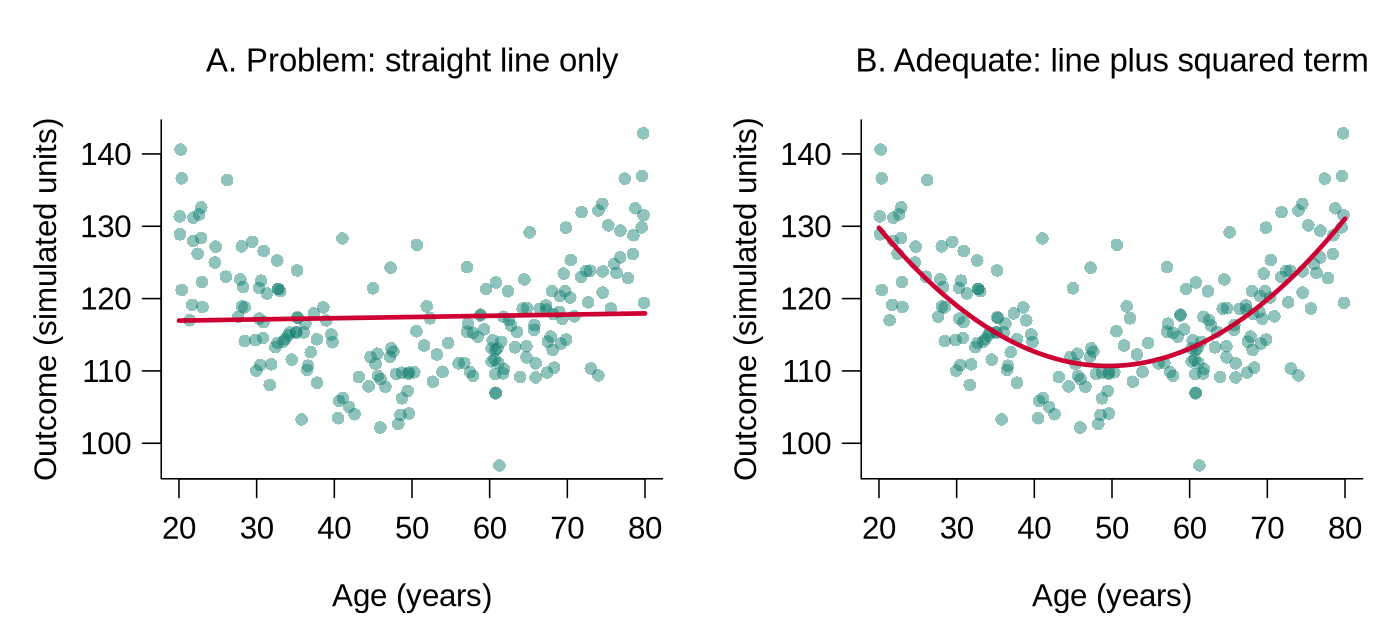
age_ctsq) lets the fitted line bend, so it follows the data. In bp01.csv the relationship between age and systolic pressure is close to a straight line, so the squared term adds little there; having it ready makes the check quick to run.SPSS is a statistics package that is often used through menus. A workflow built only by clicking through menus, in SPSS or any similar program, is difficult to re-derive unless the underlying commands are also saved (SPSS calls them syntax). A script can be re-run six months from now, by a colleague, on a different computer.
A versioned and logged set of files records how the dataset has changed. The variables within each file need the same care.
5.4 Naming Variables and Keeping a Codebook
Even a relatively focused study can give rise to a large number of variables once transformed and recoded variables have been created, so the names and their documentation need a system. The first tab below sets out the naming convention and the second applies it to age; open both to see the rule and the example side by side.
Use short but informative names and have all related variables start with the same name. Long names can be shortened by removing vowels (e.g., wtr_cstrn for “water cistern”). If your statistics program is case sensitive, use ONLY lower-case letters. At some point, prepare a master list of all variables.
Table 1.6 applies the naming convention to age: each variable derived from age begins with the same name.
Table 1.6. The original age variable and four variables derived from it, all named to begin with age.
| Variable | Description |
|---|---|
age | Original data (in years) |
age_ct | Age after centring by subtraction of the mean |
age_ctsq | Quadratic term (age_ct squared) |
age_c2 | Age categorised into 2 categories (young vs old) |
age_c3 | Age categorised into 3 categories |
Because each name derived from age begins with age, the related variables sort together and the link between them is obvious. The names are half of the documentation, and the codebook is the other half.
A codebook (also called a data dictionary) lists every variable with its meaning, type, units, allowed values, and number of missing values, so that a collaborator can use the file without asking the original analyst. Table 1.7 is the codebook for bp01.csv, extended with the four variables derived in the cleaning script. The ranges and missing counts come from the verification checks in the next section.
Table 1.7. Codebook for bp01.csv, extended with the four variables derived in the cleaning script.
| Variable | Description | Type and units | Values or range | Missing |
|---|---|---|---|---|
id | Participant identifier | text | BP0001 to BP1092, one per participant | 0 |
age | Age | number, years | 18 to 85 | 11 |
sex | Sex | text (factor in analysis) | Female, Male | 0 |
smoker | Smoking status | text (factor in analysis) | No, Yes | 0 |
bmi | Body mass index | number, kg/m² | 16.0 to 41.2 | 0 |
systolic | Systolic blood pressure | number, mmHg | 85 to 186 | 18 |
diastolic | Diastolic blood pressure | number, mmHg | 42 to 119 | 19 |
on_treatment | Takes blood-pressure medication | text (factor in analysis) | No, Yes | 0 |
age_ct | Age minus the mean age of 48.05 (derived) | number, years | −30.05 to 36.95 | 0 |
age_ctsq | age_ct squared (derived) | number | 0 to about 1365 | 0 |
age_c3 | Age band (derived) | factor | young (18 to 35), middle (36 to 55), older (56 to 85) | 0 |
htn | Hypertension by the 140/90 rule (derived) | factor | normotensive, hypertensive | 0 |
The missing counts refer to bp01.csv; in the cleaned file every variable is complete because the 45 incomplete records were removed. A codebook is updated each time a variable is added or redefined, and saving it as a .csv file beside the data (as shown in Activity 1.3 in the next section) keeps the two together.
This section has set out how raw responses are coded and entered, how each version of a file is named, stored and logged, and how variables are named and documented in a codebook. The key takeaways below draw the section together before its knowledge check.
Key Takeaways
- 4.1 Careful coding prevents errors that would otherwise cascade through the whole analysis, and three rules do most of the work: give missing values a code that can never be a real response (such as −999), use numeric codes listed in a master list or codebook, and store only one piece of information in each variable. When you receive someone else’s file, read it alongside its data dictionary and look for the five common faults: a missing code that could be a real value (99 for a refused age), text in a numeric field (“none” in a count of hours), a compound code, mixed date formats, and missing values recorded in different ways (a blank in one row, 99 in another). For each fault, state both the problem and the correction: an impossible missing code that is converted to
NA, the number the text means, two separate variables, one unambiguous date format such as YYYY-MM-DD, and one documented missing-value convention. A common trap is to propose fixing the raw file by hand; every correction belongs in the cleaning script, which reads the raw file and writes a new version. Remember also that splitting a compound code splits its missing code, so a 99 becomes a 9 in each new variable and later shows up as an unexpected category. - 5.2 Typing data from paper forms into a computer is where many small errors creep in, so plan the entry step rather than leaving it to chance. The strongest defence is double data entry: two people enter the same forms independently and a program compares the two files, as
anti_join()does in Worked Example 1.6, so that each disagreement can be checked against the original form. Double entry cannot catch an error that both people make in the same way, so it reduces errors substantially without removing every one. Use spreadsheets with great caution, because sorting a single column scrambles the rows and can ruin a dataset in one step, and save and back up the original files as soon as entry ends. When you assess an entry plan in a question, look for these three elements (double entry with a programmed comparison, care with spreadsheets, and an immediate backup) and name any that are missing. - 5.3 Files multiply quickly during a project, so give them a system from the start. Name each file logically with a two-digit suffix (such as
bp01.csv,bp02.csv), save every change as the next version rather than overwriting the last one, keep the raw data read-only in their own folder (data/raw) apart from the processed data (data/processed), and keep a short file log that records what changed and how many observations and variables each version holds. The pay-off is that if you find a cleaning error three steps later, you can rebuild the file from the untouched raw version by rerunning the script. When you read a file log such as the blood pressure example in 5.3, check that each entry says what was done and that its counts match what R reports for that version (nrow()gives 1092 rows forbp01.csvand 1047 for the cleaned file). The fault to look for in a question is a plan that edits and saves over the working file, or that keeps raw and cleaned data in the same place. - 5.4 Even a small study ends up with many variables once recoded and derived ones are added, so naming and documentation matter. Use short, informative, lower-case names, and start related variables with the same stem, so that
age,age_ct,age_ctsqandage_c3sort together and their link is obvious. Keep a codebook (data dictionary) that lists every variable with its meaning, type, units, allowed values and number missing, as Table 1.7 does for the blood pressure study, and update it whenever you add or redefine a variable; it is often more useful to a collaborator than the code itself. A good test is whether a collaborator could open the file and the codebook and use the data without asking you a single question. The codebook is also your reference when you check data: a value or category in the file that the codebook does not allow is a fault to explain.
1. A school board sends you a survey file in which pa_days records the number of days in the past week on which a student was active for at least 60 minutes, so its real values run from 0 to 7. The data dictionary supplied with the file states “0 = question not answered”. Which statement identifies the coding fault and the best-practice correction?
pa_days mixes inactive students with students who skipped the question; the rule is a missing code that can never be a real response, recorded in the codebook and converted to NA in the script, never by hand in the raw file. Option (c) is tempting, but na.rm = TRUE drops only values that are already NA; R treats every 0 as a real zero, so the non-answers would still pull the mean down. (Section 2, slide “Three rules that prevent cascading errors”, 4.1.2 Spotting Coding Faults in a Raw File and Worked Example 1.4; Objective 4.1)2. A diabetes clinic file stores dtype_ins, a two-digit code whose first digit is the type of diabetes (1 = type 1, 2 = type 2) and whose second digit is insulin use (1 = yes, 2 = no), so 21 means type 2 diabetes treated with insulin; 99 means missing. Which correction follows best practice?
dtype_ins packs two facts into one value, so any analysis of insulin use alone, or of diabetes type alone, first has to take the variable apart; splitting it gives two variables that can each be tabulated and modelled. The missing code needs care: split digit by digit, 99 becomes a 9 in each new variable, which later shows up as an unexpected category, so each new variable gets its own missing code, converted to NA. Option (a) is tempting because labels make the output readable, but the labelled variable still combines two facts, and option (b) edits the raw file by hand, which leaves no record. (Section 2, slide “Three rules that prevent cascading errors” and 4.1.2 Spotting Coding Faults in a Raw File; Objective 4.1)3. Two research assistants independently enter the same 200 forms. The comparison step, anti_join() run in both directions, returns the output below: the first table lists the rows of entry_a with no exact match in entry_b, and the second the reverse. What does the output show, and what is the next step?
> anti_join(entry_a, entry_b, by = c("id", "weight_kg", "height_cm"))
# A tibble: 1 × 3
     id weight_kg height_cm
  <int>     <dbl>     <dbl>
1    57        68       172
> anti_join(entry_b, entry_a, by = c("id", "weight_kg", "height_cm"))
# A tibble: 1 × 3
     id weight_kg height_cm
  <int>     <dbl>     <dbl>
1    57        86       172
anti_join() returns: the rows of one entry with no exact match in the other, so a record listed in both directions is one on which the two entries disagree. Here the two people typed 68 and 86 kg for the same participant, a pair of swapped digits, and only the paper form can say which is right. Option (b) is tempting because averaging seems fair, but 77 kg is a value that nobody recorded; option (d) overlooks that an error made identically by both people produces no disagreement, so double entry reduces errors substantially without removing every one. (Section 2, slide “Double-entry and the spreadsheet hazard”, 5.2 Entering the Data and Worked Example 1.6; Objective 5.2)4. An analyst cleaning flu03.csv (2,450 observations, 14 variables) corrects 31 impossible ages and saves the result over flu03.csv. Two weeks later a reviewer asks which records were changed, and the analyst cannot say. Which practice would have prevented the problem?
flu04.csv keeps flu03.csv intact, so the two versions can be compared to list the 31 changed records, the log states what changed and when, and the script can rebuild flu04.csv from flu03.csv at any time. Option (a) is tempting because the comment records that a change was made, but once flu03.csv is overwritten its earlier state is gone, so the changed records cannot be identified and the step cannot be rerun from its starting point; option (d) breaks the rule that raw data are read-only. (Section 2, slide “Versioning and the file log”, 5.3 Organising and Versioning Files and Activity 1.2; Objective 5.3)5. A collaborator receives a file whose age-related variables are named Age, AGE2, agegroup_new and x17, with a codebook that lists only the variable names. Which change best follows the conventions for naming and documenting variables?
Age and age as different names, and a codebook with meaning, type, units, allowed values and missing count lets a collaborator use the file without asking the original analyst. Option (b) is tempting because the names are short, but v1 to v4 carry no information, and option (c) gives names containing spaces, which are awkward in code and still lack units and allowed values. (Section 2, slide “Naming conventions and the master list”, 5.4 Naming Variables and Keeping a Codebook, Table 1.6 and Table 1.7; Objective 5.4)6. A youth sports-injury programme sends you its raw file, inj01.csv, with the data dictionary below. Which statement names three coding faults and corrects each according to best practice?
id   sport_sex  prev_inj  inj_date
101  11         2         07/03/2026
102  22         0         2026-03-09
103  99         1         12 Mar 26

Data dictionary as supplied
  sport_sex  first digit = sport (1 soccer, 2 hockey, 3 basketball);
             second digit = sex (1 female, 2 male); 99 = missing
  prev_inj   number of previous injuries; 0 = not reported
  inj_date   date of injury
sport_sex packs sport and sex into one value, and its missing code 99 would split into a 9 in each new variable; prev_inj uses 0, a real and common answer, as its missing code, so players with no previous injury cannot be told apart from those whose answer was not reported; and inj_date uses three formats, of which 07/03/2026 is ambiguous (7 March or 3 July). Each fix belongs in the cleaning script, which writes the next version of the file, so the raw file stays as received. Option (b) is tempting because every code is documented, but documentation cannot separate a real 0 from a missing one or undo a compound code; options (a) and (c) edit or overwrite the raw file, which leaves no record of what was changed. (Section 2, 4.1.2 Spotting Coding Faults in a Raw File and 5.3 Organising and Versioning Files; Objectives 4.1 and 5.3)Program Files, Data Editing & Verification
Overview
An earlier section organised your files and variables. This section turns to the analyses themselves: working in program mode rather than interactively (so the work is reproducible), editing data systematically rather than ad hoc, and verifying that the dataset behaves as expected before you draw any inferences from it. The discipline you build here is what separates a defensible analysis from a fragile one, and it has been argued that reproducibility can serve as a minimum standard for evaluating computational research when full independent replication is not possible (Peng, 2011).
Learning Objectives
- 1.2 Contrast interactive and program-mode workflows and justify why programs are required for reproducible work.
- 6.1 Edit data through scripted, documented steps (labelling variables and categories and converting every missing-value code to NA) rather than ad hoc fixes to the raw file.
- 6.2 Run systematic verification checks on ranges, types, and internal consistency, and use their output to identify implausible values and unexpected categories.
- 6.3 Decide when verification is sufficient to move on to substantive analysis.
1.2 Program Mode and Interactive Mode
Statistical programs can be used in an interactive mode (selecting items from menus or typing in a command) or in program mode (compiling a series of commands into a program and then running it). The difference lies in what is left behind once the work is done. In interactive mode, each command is carried out and then disappears, so the only lasting product is the result on the screen. In program mode, the commands are written into a file that is saved, which means the file itself becomes a complete list of the steps that produced the result. For example, an analyst who recodes age in the Console can see the new variable but has no saved record of the rule used, whereas an analyst who writes the recode in a script can open the file months later and read exactly how it was done.
The two modes suit different jobs, and only one of them leaves a record. Open both tabs below to compare what each mode is good for and why program mode is the one used for the real processing and analysis.
Interactive mode is very useful for exploring your data and trying out analyses. However, it should not be used for any of the “real” processing and/or analysis because it is very difficult to keep a clear record of steps taken. Consequently, it is difficult or impossible to reconstruct the analyses you have completed.
Program mode is the recommended approach. You compile the commands into a program and then run it. These program files can be saved and used to reconstruct any analyses you have carried out. Key tips: name files logically, structure the program to be easy to follow, use sequential indents, and document the file thoroughly with comments.
In RStudio, interactive mode corresponds to typing commands directly into the Console pane, or to clicking through menus such as Import Dataset, and program mode corresponds to writing the commands in a script file (.R) and running it. A practical habit combines the two: commands are tried out in the Console, and each command that is kept is copied into the script with a comment, so that the script alone can recreate every result. In R, a comment is any text that follows a # symbol on a line, and R ignores it when the code runs.
One rule follows directly from this, and it is worth remembering because breaking it is a common source of results that cannot be reproduced.
Do Every Analysis in the Statistical Program
Do all of the analyses in your statistical program. Don’t start doing basic statistics in a spreadsheet. You are going to need the statistical program eventually, and it will be much easier to keep track of all your analyses if they are all done there.
Program mode keeps a record of every step, so a result that cannot be reproduced usually points to a menu or spreadsheet step that was never saved as code. The same discipline applies to editing the data before any analysis begins.
6.1 Editing the Data in a Script
Before beginning any analyses, spend time editing your data. Three edits are the most important: labelling variables, labelling categories, and converting the missing-value codes. Click each card below to read what each edit involves and how it is made in R.
Each edit is made in the cleaning script rather than by typing into the raw file, so it can be checked and repeated. A codebook table kept beside the data gives each variable its label, factor() attaches a text label to each category code (Worked Example 1.5), and na_if() or the na argument of read_csv() converts every missing-value code to NA (Worked Example 1.4). The last edit has the largest consequences, because until it is made R treats a code such as 999 as a real value. Edited data must still be checked for errors before analysis.
6.2 Verifying the Data
Before you start any analyses, you must verify that your data are correct. By this we mean checking that every value in the file is one that could really have been recorded for that participant, and that the file contains the records it is supposed to contain. Verification matters because a model cannot tell a typing error from a real measurement; an age of 999 or a misspelled category is analysed just as faithfully as a correct value, and the error passes silently into the results. This can be combined with data processing and involves going through all of your variables, one-by-one.
The checks differ for continuous and categorical variables. Expand both panels below to see the checks for each type.
- Determine the number of valid observations and the number of missing values
- Check the maximum and minimum values (or the 5 smallest and 5 largest) to make sure they are reasonable; if they are not, find the error, correct it, and repeat the process
- Prepare a histogram of the data to get an idea of the distribution and see if it looks reasonable
- Determine the number of valid observations and the number of missing values
- Obtain a frequency distribution to see if the counts in each category look reasonable (and to make sure there are no unexpected categories)
Activity 1.3, at the end of this section, runs these checks in R on the raw blood pressure file, after a codebook that states what each variable should contain, and adds two cross-variable checks: a search for diastolic readings above the systolic reading and a count of the distinct identifiers. Table 1.8 explains how to read each check in its output and what a problem would look like.
Table 1.8. The verification checks in Activity 1.3: what the output shows for bp01.csv and what would signal a problem.
| Check | What the output shows for bp01.csv | What would signal a problem |
|---|---|---|
1. summary() | Min. and Max. are the smallest and largest values; 1st Qu., Median, and 3rd Qu. split the data into quarters; and NA's counts missing values. Ages run from 18 to 85, BMI from 16.0 to 41.2, systolic pressure from 85 to 186 mmHg, and diastolic pressure from 42 to 119 mmHg, all of which are possible in adults. | A minimum or maximum that cannot be true, such as an age of 999 or a blood pressure of 0, or a mean far from the median, would call for a closer look. |
2. colSums(is.na()) | is.na() marks each missing value as TRUE and colSums() counts the TRUE values in each column: 11 ages, 18 systolic values, and 19 diastolic values are missing, and the other variables are complete. | Missing counts that differ from the study records, or missing values in a variable that should be complete, would need explaining. |
3. head(sort()), tail(sort()) | sort() puts the values in order, head(..., 5) shows the first five, and tail(..., 5) the last five. The lowest systolic value (85 mmHg) and the highest age (85 years) fill all five places shown. A count with sum(bp_raw$systolic == 85, na.rm = TRUE) finds 15 participants at 85 mmHg, and the same count for age finds 6 participants aged 85. | An impossible value would be an error. A pile-up of identical values at the edge, as here, can also mean that values beyond a limit were recorded as the limit, which the study protocol should confirm. |
4. hist() | The histogram of systolic pressure is a single hump centred near 128 mmHg. The small bars above 180 mmHg hold three high but possible readings (181, 186, and 186 mmHg). | An isolated bar far from the rest, or a shape that contradicts what is known about the variable, would need investigation. |
5. table(..., useNA = "ifany") | Each category is listed with its count. The argument useNA = "ifany" adds an NA column only when values are missing, and none are missing here. | An unexpected category, such as a misspelling, or more missing values than expected would need correcting. |
6. filter(diastolic > systolic) | filter() keeps the rows that meet the condition. The result has 0 rows, so no participant has a diastolic reading above the systolic reading. | Any returned row identifies a record to check against the original form. |
7. n_distinct(id) | n_distinct() counts the different values. There are 1092 identifiers for 1092 rows, which confirms one row per participant. | Fewer identifiers than rows would mean duplicated records or repeated measurements that the codebook should explain. |
The histogram is often the quickest way to spot a planted code. A histogram divides the range of a variable into equal intervals and draws a bar for the number of values in each, so its horizontal axis must stretch from the smallest value to the largest. If a missing-value code such as 999 has been left in an age variable, the axis has to reach all the way to 999, which squeezes the real ages into a narrow block at one end and leaves a small isolated bar far away from them. The shape is so unusual that the problem is visible at a glance, even when only a few values carry the code. Figure 1.4 shows three histograms of the kind hist() produces: one of plausible values, one with a planted missing-value code, and one with a long right tail.
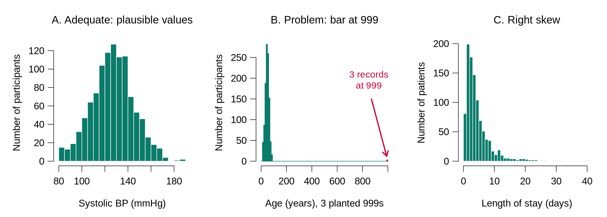
hist() produces. A. Systolic blood pressure in bp01.csv: a single hump of plausible values. B. A copy of bp01.csv in which three missing ages were stored as 999 (planted for illustration): the real ages are squeezed against the left edge, and an isolated bar appears at 999 (highlighted in red here). C. Simulated hospital length of stay: most values are small and a long tail stretches to the right. A skewed shape like C can be correct for the variable; it still matters for later choices, such as the log transformation discussed in the next section.A check that finds a problem leads to a fix in the cleaning script, after which the check is run again.
Reading the fix in Activity 1.3. The raw file passes every check above, so the activity plants three typical errors on a copy of the data, leaving the raw file untouched, and fixes them in the cleaning script. na_if(age, 999) turns the code into NA. case_when() checks each condition in turn: %in% asks whether the value is one of the listed spellings, and the value after ~ is assigned when it is. Any value that matches no condition becomes NA, so a spelling that the analyst did not anticipate appears as missing in the next frequency table and is never silently relabelled. After the fix, the counts of 554 women and 538 men match the raw file, and age has 14 missing values (11 original and 3 converted); where possible, the three ages are looked up on the original forms and entered through the script. The activity's codebook is a table built with tribble(); saved as a .csv file in the data folder, it stays with the data, any collaborator can open it in R or in a spreadsheet, and it is updated in the same session whenever a variable is added or redefined in the cleaning script.
Each fix is therefore an edit of the kind described in 6.1, found by a check of the kind described here. The remaining question is when the checking can stop.
6.3 Deciding When Verification Is Complete
Verification could go on indefinitely, so the analyst needs a clear point at which to move on to substantive analysis. The checklist below states that point; learn its items, and work through them one at a time whenever you judge whether a dataset is ready.
Verification Checklist: When to Move On
Verification can be considered complete when every statement below is true, and each fix has been made in the cleaning script and recorded in the log.
- Every variable in the file appears in the codebook, with its meaning, type, units, and allowed values.
- The number of rows matches the number of participants (or records) expected from the study records, and every identifier is unique.
- For each continuous variable, the number of missing values is known, and the smallest and largest values are possible.
- Each continuous variable’s histogram shows no isolated bar at a code such as 999 and no shape that contradicts what is known about the variable.
- For each categorical variable, the frequency table shows only the categories listed in the codebook.
- Every missing-value code has been converted to NA.
- Cross-variable checks, such as a search for diastolic readings above the systolic reading or for pregnancies recorded among male participants, return no rows, or every returned row has been checked against the original form.
- The cleaning script runs from top to bottom on the raw file and reproduces the cleaned file exactly.
If any item fails, the fix is made in the script and recorded in the log, and the checks are run again, which is the iterative loop of the workflow applied to verification. Activity 1.3 practises the whole sequence on bp01.csv: it builds a codebook, runs the checks of Table 1.8, then plants three typical errors on a copy of the file, finds them with the same checks and fixes them in the cleaning script. Run it along with the reading, then answer the questions from your own output.
bp01.csv
Text version of the activity: the code of the run-along script, its console output and notes on reading it.
library(dplyr)                    # part of the tidyverse
bp_raw <- read.csv("https://heal-learn.ca/r-activities/data/bp01.csv")   # course data, read from the website
nrow(bp_raw) # number of rowsThe file is read straight from the course website into bp_raw, which is never changed. It has 1092 rows, which should be one per participant. Line 7 loads dplyr, one of the tidyverse packages, for tribble(), filter(), n_distinct(), mutate(), na_if() and case_when(); its messages about masked objects are normal.
codebook <- tribble(
  ~variable,      ~label,                             ~units_or_codes,
  "id",           "Participant identifier",           "BP0001 to BP1092",
  "age",          "Age",                              "years",
  "sex",          "Sex",                              "Female, Male",
  "smoker",       "Smoking status",                   "No, Yes",
  "bmi",          "Body mass index",                  "kg/m2",
  "systolic",     "Systolic blood pressure",          "mmHg",
  "diastolic",    "Diastolic blood pressure",         "mmHg",
  "on_treatment", "Takes blood-pressure medication",  "No, Yes"
)
codebookLabelling variables is the first component of data editing. tribble() builds a small table row by row: the first line names the columns, each name starting with ~, and every following line describes one variable. In a project, the codebook is saved as a .csv file beside the data (for example with write_csv()), where any collaborator can open it, and it is updated in the same session whenever the cleaning script adds or redefines a variable. Category labels are attached separately with factor(), as shown in Worked Example 1.5 (Section 2).
summary(bp_raw[, c("age", "bmi", "systolic", "diastolic")])
colSums(is.na(bp_raw))            # number missing in every variable
head(sort(bp_raw$systolic), 5)    # the five smallest values
tail(sort(bp_raw$systolic), 5)    # the five largest values
head(sort(bp_raw$age), 5)
tail(sort(bp_raw$age), 5)
sum(bp_raw$systolic == 85, na.rm = TRUE)   # how many at the lowest value?
sum(bp_raw$age == 85, na.rm = TRUE)        # how many at the highest age?
hist(bp_raw$systolic, breaks = 30, xlab = "Systolic BP (mmHg)", main = "")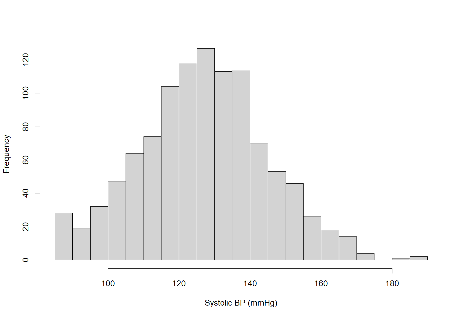
Reading the checks. In summary(), Min. and Max. are the smallest and largest values, 1st Qu., Median and 3rd Qu. split the data into quarters, and NAs counts missing values. Ages run from 18 to 85, BMI from 16.0 to 41.2, systolic pressure from 85 to 186 mmHg and diastolic pressure from 42 to 119 mmHg, all possible in adults. colSums(is.na()) counts the missing values: 11 ages, 18 systolic and 19 diastolic values, which are noted and explained rather than treated as errors. sort() puts the values in order and head(..., 5) and tail(..., 5) show the first and last five: the lowest systolic value (85 mmHg, 15 participants) and the highest age (85 years, 6 participants) fill all five places. A pile-up at the edge can mean that values beyond a limit were recorded as the limit, which the study protocol should confirm. The histogram is a single hump centred near 128 mmHg, and the three small bars above 180 mmHg hold high but possible readings (181, 186 and 186 mmHg).
table(bp_raw$sex, useNA = "ifany")
table(bp_raw$smoker, useNA = "ifany")
table(bp_raw$on_treatment, useNA = "ifany")
bp_raw |> filter(diastolic > systolic)    # should return no rows
n_distinct(bp_raw$id) # compare with nrow()Each frequency table lists only the categories in the codebook; useNA = "ifany" adds an NA column only when values are missing, and none are. filter() keeps the rows that meet the condition: no participant has a diastolic reading above the systolic reading. n_distinct() counts the different identifiers: 1092 for 1092 rows, so there is one row per participant. Fewer identifiers than rows would mean duplicated records or repeated measurements that the codebook should explain.
bp_bad <- bp_raw                       # a copy; bp_raw is untouched
bp_bad$age[c(5, 120, 640)] <- 999      # planted: unknown age typed as 999
bp_bad$sex[c(10, 302)] <- "F"          # planted: abbreviation
bp_bad$sex[450] <- "male"              # planted: lower-case spelling
summary(bp_bad$age)
tail(sort(bp_bad$age), 5)
hist(bp_bad$age, breaks = 30, xlab = "Age (years)", main = "")
table(bp_bad$sex, useNA = "ifany")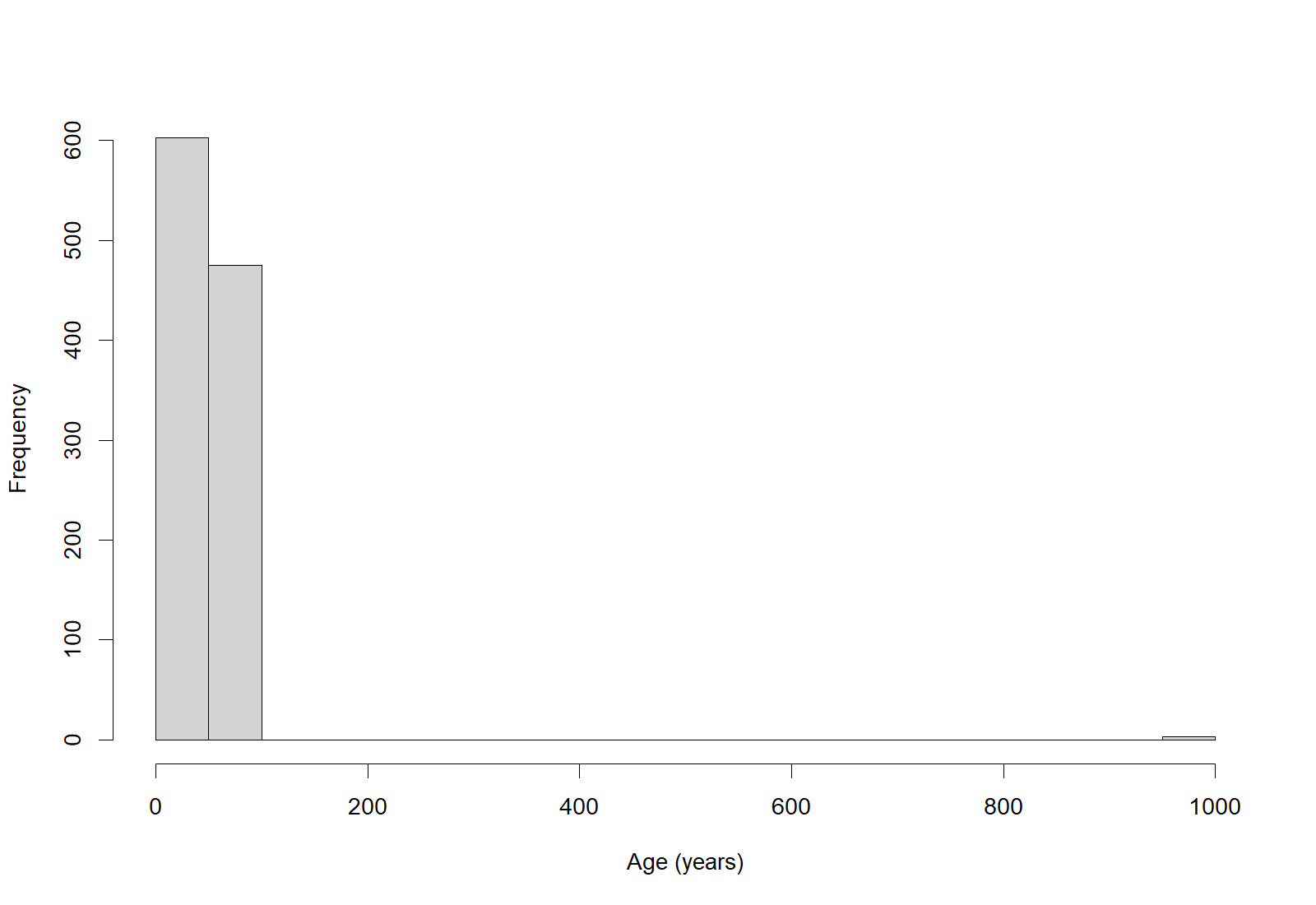
The three planted ages of 999 make the maximum 999 and raise the mean from 48.05 to 50.69 while the median stays at 49; the five largest values and the isolated bar in the histogram show them. The frequency table shows four categories where the codebook allows two: "F" (2) and "male" (1) are other spellings of Female and Male. The 11 missing ages are the original missing values, not a new problem.
bp_fixed <- bp_bad |>
  mutate(age = na_if(age, 999),
         sex = case_when(sex %in% c("Female", "F") ~ "Female",
                         sex %in% c("Male", "male") ~ "Male"))
Reading the fix. na_if(age, 999) turns the code into NA. case_when() checks each condition in turn: %in% asks whether the value is one of the listed spellings, and the value after ~ is assigned when it is. Any value that matches no condition becomes NA, so a spelling that the analyst did not anticipate appears as missing in the next frequency table and is never silently relabelled. After the fix, age has 14 missing values (11 original and 3 converted) and sex has 554 women and 538 men, as in the raw file; where possible, the three ages are looked up on the original forms and entered through the script, and each rule is recorded in the cleaning log.
R Reflect on what you just ran
Answer each question from your own output, as on the midterm: compare each value with what is possible and with the codebook, decide what to do about each problem, and write the rule you would record in the cleaning log.
1. Lines 26 to 41 are a first verification pass of the raw file. Using their output, judge whether bp01.csv is ready for analysis: state whether each minimum and maximum is possible and what the counts of missing values (NAs) mean, explain what the pile-up of values at 85 could mean, and state what the frequency tables, the consistency check (line 40) and the identifier count (line 41) show.
NAs (11 ages, 18 systolic and 19 diastolic values) are missing values already coded as NA; they are counts to note and explain, not errors. The five smallest systolic values and the five largest ages are all 85 (15 people at 85 mmHg and 6 aged 85); these values are possible, but a pile-up at the edge can mean that values beyond a limit were recorded as the limit, so the study protocol should confirm it. The histogram is a single hump centred near 128 mmHg, and the three readings above 180 mmHg (181, 186 and 186) are high but possible. Each frequency table shows only the codebook categories, with no NA; no participant has a diastolic reading above the systolic one (0 rows); and 1092 identifiers for 1092 rows confirm one row per participant. The file therefore passes this first verification pass, and no value needs to be changed.2. Suppose you had received bp_bad as the raw file. The output of lines 48 to 51 reveals two problems, one in each of two variables (the 11 missing ages are not one of the problems). Identify the two problems, and for each state whether you would keep, transform, or exclude the affected values, and write the rule you would record in the cleaning log.
NA, keeping the rows, unless the true age can be recovered from the original form, in which case it is corrected. Log rule, for example: age = 999 (n = 3) lies outside the possible range and is the code for an unknown age; values checked against the forms; unverifiable values set to NA; rows retained. Problem 2 is in sex: the frequency table shows four categories where the codebook allows two, and “F” (n = 2) and “male” (n = 1) are other spellings of Female and Male. Decision: keep the values and recode them to the codebook labels, because their meaning is clear; a transformation does not address either problem, because a miscoded value is an error to be corrected. Log rule, for example: sex “F” (n = 2) recoded to Female and “male” (n = 1) to Male, to match the codebook; rows retained.3. Run your own code: at the end of the script, type summary(bp_fixed$age) and table(bp_fixed$sex, useNA = "ifany") and run them. Use the output to show that the fix worked. A colleague says it would be quicker to open bp01.csv in a spreadsheet and type the corrections there: do you agree? State how the corrections should be made, according to best practice, and what the cleaning log should record.
NA values plus the 3 converted codes. Sex now has only the two codebook categories, 554 Female and 538 Male, which match the raw file, and no NA, so every spelling was matched by case_when(). I disagree with the colleague: corrections are made in a script that reads the raw file and writes a new version, never by editing the raw file by hand. The raw file then stays untouched, every change is written down where a reviewer can check it, and rerunning the script repeats every step exactly; a hand edit in a spreadsheet leaves no record, so the cleaned file cannot be reproduced. The cleaning log records each rule with its count (age 999 set to NA, n = 3; sex “F” recoded to Female, n = 2, and “male” to Male, n = 1), and where possible the three ages are looked up on the original forms and entered through the script.Your output from Activity 1.3 shows the three habits of this section working together: the checks run as a script, the problems they reveal are fixed by scripted edits, and the checklist decides when the file is ready. The key takeaways below draw the section together before its knowledge check.
Key Takeaways
- 1.2 R and other statistical programs can be used in two ways. In interactive mode you type commands into the Console or click through menus, which is handy for exploring and trying things out but leaves no reliable record of what you did. In program mode you write the commands in a saved, commented script (an
.Rfile) and run it, so the script becomes the honest record that lets you, or a colleague on another computer six months later, rerun, check and share every step. A practical habit is to try a command in the Console and, once you decide to keep it, copy it into the script with a comment, and to do every analysis, even basic statistics, in the statistical program rather than in a spreadsheet. If a question asks why a result cannot be reproduced, look for a point-and-click or spreadsheet step that was never saved as code. - 6.1 Before any analysis the data are edited, and that editing happens in the cleaning script, never by typing into the raw file. Three edits matter most: give every variable a descriptive label (for example, in a codebook table saved beside the data), give every category code a text label (for example, with
factor(), so that 1 and 2 print as Female and Male), and convert every missing-value code (999, a blank, a full stop) to the single code the software treats as missing, which isNAin R. The last edit has the biggest consequences, because until it is made R treats a code such as −999 as a real number and averages it with the real values, as Worked Example 1.4 shows. You can make the conversion withna_if()or with thena =argument ofread_csv(). When you describe an edit in an answer, say what was changed, which step of the script changed it, and that the raw file was left untouched. - 6.2 Verification means going through your variables one by one to confirm that the data are correct before you trust any result. For a continuous variable, check the numbers of valid and missing values, the smallest and largest values (or the five smallest and five largest, with
head(sort())andtail(sort())) and a histogram; for a categorical variable, check the valid and missing counts and a frequency table, such astable(x, useNA = "ifany"). Add cross-variable checks, such as a search for diastolic readings above systolic ones, and confirm that every identifier is unique. When you readsummary()ortable()output in a question, compare each minimum, maximum and category with what is possible and with what the codebook allows: a maximum age of 999, a mean far from the median, or a category such as “F” or 9 that the codebook does not list is an error to trace. Each problem is corrected in the script and the check is run again, while a count of missing values (NA's) is something to note and explain rather than, by itself, an error. - 6.3 It can be hard to know when you have checked enough, so the verification checklist in 6.3 gives you a clear point at which to move on. Verification is complete when every variable is in the codebook, the number of rows matches the study records and every identifier is unique, every minimum, maximum and category is possible, no histogram shows an isolated bar at a code such as 999, every missing code has become
NA, cross-variable checks return no unexplained rows, and the cleaning script runs from top to bottom on the raw file and reproduces the cleaned file exactly. If any item fails, fix it in the script, record it in the log and run the checks again. When a question asks whether a dataset is ready for analysis, work through the checklist item by item and name the first item that is not yet met.
1. Two analysts produce the same table of smoking prevalence by age group. Analyst A typed commands into the RStudio Console and copied the counts into a spreadsheet to work out the percentages. Analyst B wrote a saved, commented .R script that reads the raw file, cleans it and produces the table. A reviewer then finds a duplicated record in the raw file. Which statement is correct?
2. The data dictionary for smoke_status lists 1 = never, 2 = former, 3 = current and 999 = missing. The first frequency table from the raw file is shown below; <NA> counts blank cells. Which editing step is correct?
> table(raw$smoke_status, useNA = "ifany")

   .    1    2    3  999 <NA>
  14  402  233   97    9   21
NA, and attaches text labels to the codes so that output reads never, former and current rather than bare numbers. Option (a) is tempting because it follows the dictionary to the letter, but a full stop is another missing-value convention, not a smoking category; option (d) edits the raw file by hand, which leaves no record of the change. (Section 3, slide “Three components of scripted editing” and 6.1 Editing the Data in a Script; Objective 6.1)3. A school health survey enrolled students aged 12 to 17, and sleep_hrs records each student’s usual hours of sleep per night. The first verification pass gives the output below. Which conclusion follows?
> summary(dat[, c("age", "sleep_hrs")])
      age         sleep_hrs
 Min.   :12.0   Min.   : 5.00
 1st Qu.:13.0   1st Qu.: 7.00
 Median :15.0   Median : 8.00
 Mean   :14.6   Mean   :10.84
 3rd Qu.:16.0   3rd Qu.: 9.00
 Max.   :17.0   Max.   :99.00
                NA's   :6
tail(sort(dat$sleep_hrs), 5) to list the extreme values, a check of each against the source, a fix in the script and a repeat of the check, because where there is one error there are often more. Option (b) is tempting because some variables do have a long right tail (Figure 1.4, panel C), but here the cause is an impossible value, an error to correct rather than a shape to transform. (Section 3, slide “Check before you trust”, 6.2 Verifying the Data and Table 1.8; Objective 6.2)4. A diabetes clinic file stored a two-digit code (first digit diabetes type, second digit insulin use; 99 = missing), which the cleaning script has split into dtype (1 = type 1, 2 = type 2) and insulin (1 = yes, 2 = no). The frequency table of the new dtype variable is shown below. What does it reveal, and what should the cleaning script do?
> table(clin$dtype, useNA = "ifany")

  1   2   9
 84 391  17
dtype (1 and 2) and how the variable was made. A frequency table is checked for categories that the codebook does not allow, and 9 is one; splitting 99 digit by digit gives a 9 in each new variable, so these 17 patients are the ones whose original code was missing, and their insulin values will also be 9. Option (b) is tempting because missing values usually appear as NA, but these ones are hidden behind a number, which is why every missing code must be converted; option (d) treats an error as a real but rare category. (Section 3, slide “Check before you trust” and 6.2 Verifying the Data; Section 2, 4.1.2 Spotting Coding Faults in a Raw File; Objective 6.2)5. An analyst has run summary(), histograms and frequency tables on every variable of a 1,200-row file, and every range and category is possible. Which further finding means that verification is not yet complete?
6. A district health office surveyed 500 households about their drinking water. The codebook lists hh_size (number of people in the household; 999 = not answered), kids_u5 (how many of those people are children under 5) and water_src (1 = municipal tap, 2 = private well, 3 = bottled water). The verification output is shown below; its last two lines convert the 999 codes to NA and print the mean household size again. Which reading of the output is correct?
> summary(hh[, c("hh_size", "kids_u5")])
    hh_size          kids_u5
 Min.   :  1.00   Min.   :0.000
 1st Qu.:  2.00   1st Qu.:0.000
 Median :  3.00   Median :0.000
 Mean   : 12.96   Mean   :0.526
 3rd Qu.:  4.00   3rd Qu.:1.000
 Max.   :999.00   Max.   :4.000
> sum(hh$hh_size == 999)
[1] 5
> sum(hh$kids_u5 > hh$hh_size)
[1] 3
> table(hh$water_src, useNA = "ifany")

   1    2    3   22 <NA>
 296  142   49    3   10
> hh <- hh |> mutate(hh_size = na_if(hh_size, 999))
> mean(hh$hh_size, na.rm = TRUE)
[1] 3
na_if() turns them into NA, mean(..., na.rm = TRUE) gives 3, the figure to report. The cross-variable check counts three impossible households, and the frequency table shows a category that the codebook does not list. Each problem is checked against the questionnaire, fixed in the script and checked again. Option (a) is tempting because missing values look like a problem, but a count of NA values is something to note and explain, not by itself an error; option (c) treats errors as real values, and option (d) edits the raw file by hand, which leaves no record. (Section 3, slide “Check before you trust”, 6.2 Verifying the Data, Table 1.8 and the verification checklist in 6.3; Objectives 6.1 and 6.2)Data Processing & Unconditional Associations
Overview
Earlier sections produced a verified, well-documented dataset. This section finally takes the step every student is impatient to make: the actual analysis. It begins with the analytic log that records every decision, then shows how to process outcome and predictor variables for analysis, how to recognise a multilevel data structure, and how to run the “unconditional associations” (single-predictor descriptions) that are the necessary first look at any dataset before you touch a multivariable model.
Learning Objectives
- 5.5 Keep an analytic log that allows you to reconstruct every decision you made.
- 7.1 Process outcome variables to fit the planned analysis (categorical, continuous, and count or rate).
- 7.2 Process predictor variables, including decisions about missing values, sparse categories, categorisation, scaling, and recoding.
- 7.3 Recognise multilevel structure in your dataset and the implications for later modelling.
- 7.4 Choose, run and interpret the unconditional (single-predictor) association for each pair of variable types as the first analytic step, and explain what it shows about functional form, collinearity and confounders.
5.5 Keeping an Analytic Log
Before starting the more substantial analysis, set up a system for keeping track of your results, because every processing decision in this section will have to be reconstructed later, by you, a co-author or a reviewer. Three habits make up the system: analysing in blocks, keeping log files, and labelling and dating every output. Click each card below to read what each habit involves and how it is done in R.
The log records what each run produced and also what it decided and why. Each processing step below ends in a decision of that kind, such as excluding participants with missing values or merging a sparse category, and Worked Example 1.9 shows a complete log entry for one of them. A good test of the system is whether you, three months from now, could trace any number in a report back to the script, the file version and the decision that produced it.
7.1 Processing the Outcome Variables
The type of outcome sets the type of model, so each outcome is checked against the analysis that has been planned for it before any model is fitted.
7.1.1 Outcome Types and Their Checks
While verifying data, you can also start processing your outcome variable(s). Review the stated goals of the study to determine the format(s) which best suits the goal(s). The questions to ask depend on the type of outcome; expand each panel below for the questions that apply to a categorical, continuous, and count or rate outcome.
Is the distribution of outcomes across categories acceptable? For example, if you planned a multinomial regression with a 3-category outcome, but very few observations fall in one of the categories, you might want to recode it to a 2-category variable.
Does the variable have the characteristics necessary for the planned analysis? If linear regression is planned, is the distribution approximately normal? If not, explore transformations. Note: It is the normality of the residuals which is ultimately important, but if the original variable is far from normal and there are no strong predictors, the residuals are unlikely to be normal. The reason is that a residual is what is left of each outcome value once the model’s prediction has been subtracted. When the predictors explain a large part of the outcome, the residuals can look quite different from the outcome itself. When the predictors explain little, however, each prediction stays close to the overall mean, so the residuals are little more than the outcome shifted to centre on zero, and they inherit its skew. Checking the outcome at this stage therefore gives an early warning of a problem that the residuals are likely to show later.
If Poisson regression is planned, are the mean and variance of the distribution approximately equal? The Poisson model assumes they are; when the variance runs well above the mean (a pattern called overdispersion), the fitted standard errors come out too small and the p-values look stronger than the data warrant. This happens because the model calculates its standard errors from the variance it assumes rather than from the variance the data actually show. If the counts are far more spread out than the model expects, the model believes its estimates are more precise than they really are. If that happens, consider negative binomial regression or alternative analytic approaches.
Table 1.9 gathers the outcome types from the slide and the panels above, with an example of each, the model usually used, and the check to make now. The checks in the fourth column belong to this lesson.
Table 1.9. Outcome types, with an example of each, the usual model, and the check to make now.
| Outcome type | Example | Usual model | What to check now |
|---|---|---|---|
| Binary (two categories) | Hypertensive or normotensive (htn) | Logistic regression | Both categories should contain a reasonable number of people, because a rare category gives unstable estimates. |
| Categorical with three or more categories | Smoking status recorded as never, former, or current | Multinomial regression (unordered) or ordinal regression (ordered) | The count in each category should be checked, and categories that hold only a handful of people can be combined. |
| Continuous | Systolic blood pressure in mmHg | Linear regression | A histogram should show no strong skew; if it does, a transformation such as the logarithm can be tried, and the residuals are checked after the model is fitted. |
| Count or rate | Number of clinic visits in a year | Poisson regression, or negative binomial regression when the variance is much larger than the mean | The mean and the variance of the counts should be compared, and the check is repeated after the model is fitted, because the Poisson assumption applies to people who share the same values of the predictors. |
Three terms used in the panels and in Table 1.9 need plain definitions. Table 1.10 gives the plain-language meaning of variance, residual and overdispersion.
Table 1.10. Plain-language definitions of variance, residual, and overdispersion.
| Term | Plain-language meaning |
|---|---|
| Variance | Variance measures spread. It is the average of the squared distances between each value and the mean (R divides by n − 1), and its square root is the standard deviation. |
| Residual | A residual is the difference between a person’s observed value and the value the model predicts for that person (observed minus predicted). Linear regression assumes that the residuals are roughly bell-shaped around zero. |
| Overdispersion | A count outcome is overdispersed when its variance is clearly larger than its mean. The Poisson model assumes the two are about equal, so overdispersion makes its standard errors too small and its p-values too optimistic. |
The definition of variance becomes practical in the check for a Poisson model. Worked Example 1.7 applies it to clinic visits at two clinics; watch whether each printed variance is close to the mean or far above it.
Worked Example 1.7: Comparing the variance with the mean for counts
The check for a Poisson model is to compare the mean of the counts with their variance. The invented example below records clinic visits in one year for ten patients at each of two clinics; var() computes the variance.
Reading the output. Both clinics average 2.6 visits per patient, and the decision rests on comparing each printed variance with this mean. For clinic A, var() reports 2.71, the spread of the counts measured as in Table 1.10. A variance this close to the mean is what a Poisson model expects. In clinic B, most patients have no visits or one visit and two have 9 and 12, so var() reports 18.27, and the last line, var(visits_b) / mean(visits_b), prints 7.03: the variance is about seven times the mean. That pattern is overdispersion, and a negative binomial model would be the safer starting point for these counts.
The comparison of the variance with the mean is therefore the whole check: clinic A passes it and clinic B does not. For a continuous outcome, the corresponding check concerns the residuals.
7.1.2 Residuals and Transformations
A residual is easiest to understand in a picture. Panel A of Figure 1.5 fits a straight line for systolic pressure against age in the cleaned blood pressure data and draws, for 25 randomly chosen participants, the vertical distance between each observed value and the line. Panel B collects the residuals of all 1047 participants in a histogram; a roughly bell-shaped histogram centred on zero is what linear regression assumes. Residuals are checked after a model is fitted. At the processing stage the analyst looks at the outcome itself, because a strongly skewed outcome rarely produces bell-shaped residuals.
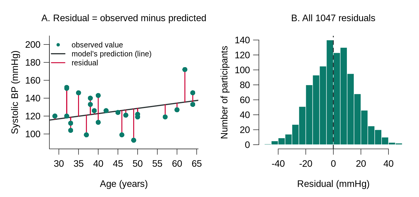
bp01.csv after cleaning). A. Each red segment is one participant’s residual, the observed value minus the value on the fitted line; points above the line have positive residuals. B. Histogram of all 1047 residuals, centred on zero (dashed line) and roughly bell-shaped, which is the pattern linear regression assumes.When the outcome itself is strongly skewed, a transformation can bring it closer to symmetry. Worked Example 1.8 shows how a log transformation changes a simulated outcome with a long right tail, hospital length of stay; compare the mean and the median before and after the transformation.
Worked Example 1.8: Before and after a log transformation
When an outcome has a long right tail, taking the natural logarithm of each value, log() in R, often makes the distribution close to symmetric, because the logarithm shrinks large values much more than small ones. The simulated example below uses hospital length of stay in days. The function rlnorm() draws right-skewed values for the simulation, and round(..., 1) keeps one decimal place.
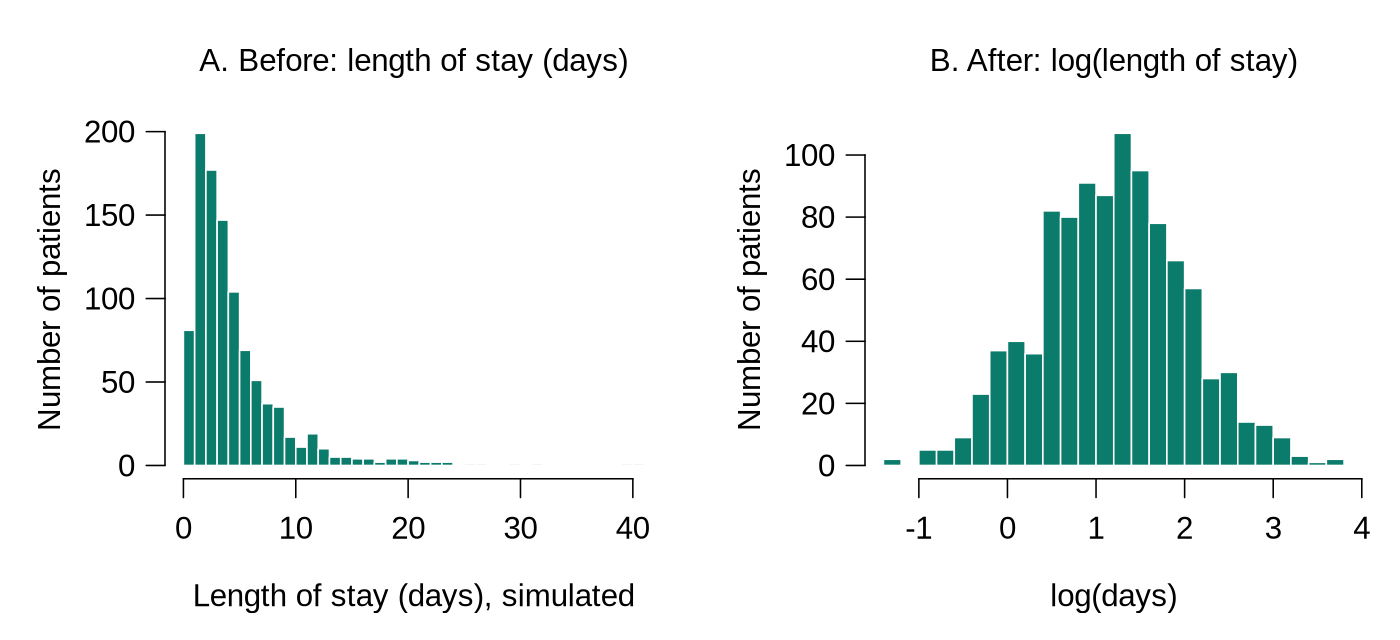
log(): the tail is pulled in and the shape is roughly symmetric.Reading the output. Before the transformation the mean (4.57 days) is well above the median (3.40 days), because the few very long stays pull the mean upwards; this gap is a quick numerical sign of right skew. After the transformation the mean (1.19) and median (1.22) are close, matching the symmetric histogram. In a real analysis the new variable is created in the cleaning script, for example mutate(log_los = log(los)), and the transformation is recorded in the codebook. The logarithm is defined only for values above zero, so an outcome that contains zeros needs adjustment first.
Once each outcome is in a form that suits the planned analysis, the same review is applied to the predictors.
7.2 Processing the Predictor Variables
It is important to go through all predictor variables to determine how they will be handled:
- Missing values: Are there many? If so, you might need to abandon plans to use that predictor, or conduct 2 analyses (one on the subset where the predictor is present and one on the full dataset ignoring the predictor). A third option, multiple imputation, fills each missing value several times with plausible values predicted from the other variables and combines the results. Whichever option is chosen is recorded in the analysis log with its reason.
- Distribution: For continuous variables, is there a reasonable representation over the whole range of values? If not, it might be necessary to categorise the variable. By this we mean that a model can describe the relationship only where there are data to support it. For example, if almost every participant smokes between 0 and 5 cigarettes a day and only a handful smoke more than 20, any estimate of what happens at high levels of smoking rests on those few people. Grouping the values into categories such as none, light and heavy keeps each part of the comparison supported by a reasonable number of participants.
- Categorical variables: Are all categories reasonably well represented? If not, you might have to combine categories.
Worked Example 1.9 applies the first item, missing values: it tabulates the missing values in the raw blood pressure file and records the resulting decision in the analytic log; notice that every number in the log entry is one that R prints.
Worked Example 1.9: Tabulating missing values and logging the decision
The first question about any predictor is how much of it is missing. The two lines below give the count and the percentage of missing values for every variable in the raw blood pressure file. colMeans(is.na()) gives the proportion missing, because R counts each TRUE as 1 and each FALSE as 0.
The decision that follows belongs in the analysis log in plain words. An entry for this file might read as follows.
The analyst writes the log entry in plain words from the counts in the output above. The number of participants excluded and its percentage also come from R: sum(!complete.cases(bp_raw)) returns 45, and round(100 * mean(!complete.cases(bp_raw)), 1) returns 4.1.
The same discipline applies to a category that holds too few people. Worked Example 1.10 combines a sparse age band in the cleaned blood pressure data; watch the count of normotensive participants in the oldest band.
Worked Example 1.10: Combining a sparse category
The cross-tabulation below splits the cleaned blood pressure data into ten-year age bands and counts normotensive and hypertensive participants in each. The breaks c(17, 29, 39, ...) work because ages are whole numbers, so the band above 17 and up to 29 holds ages 18 to 29.
Reading the output. Before merging, the 80+ band holds only 17 participants, and only 3 of them are normotensive. A logistic model that compares each band with a reference band would estimate the 80+ effect from those 3 people, which gives a very wide confidence interval: with 50–59 as the reference band, the odds of hypertension in the 80+ band are estimated at about 11 times the odds in the reference band, with a 95% confidence interval from about 3 to more than 38. A band with no normotensive participants at all would prevent the model from converging (the fitting procedure cannot settle on an answer). Merging 70–79 and 80+ into 70+ gives 24 normotensive and 49 hypertensive participants, enough for a stable estimate. The 18–29 band has only 4 hypertensive participants and might likewise be merged with 30–39. Each merge is a judgement made before the outcome model is fitted, and it is recorded in the log.
Scaling and recoding steps belong to this stage as well. Centring age (age_ct) and grouping it into bands (age_c3), for example, are made in the cleaning script and recorded in the codebook, as in Section 2. A documented choice about a predictor is defensible, whereas a predictor that is dropped, or whose missing values are filled with the mean, without saying so cannot be judged by a reader. Some datasets also hold measurements grouped within people or centres, which raises a different question.
7.3 Recognising Multilevel Data
If your data are multilevel (e.g., blood pressure measurements within individuals within centres), evaluate the hierarchical structure before any modelling. The questions to ask, and the reason they matter, are set out below.
Key Questions for Multilevel Data
What is the average (and range) number of observations at one level in each higher-level unit? Are individuals uniquely identified within a hierarchical level? It is often useful to create one unique identifier for each observation in the dataset.
Why this matters: observations from the same person, or the same centre, resemble one another more than observations drawn at random, so a model that ignores the clustering behaves as if it holds more independent information than it really does. For example, three blood pressure readings from the same person are likely to be similar, because they share that person’s genes, diet and medication; they tell the analyst less than three readings from three different people would. A model that treats every row as an independent person counts the same information several times. The result is standard errors that are too small and confidence intervals that are too narrow. Mixed models are built for exactly this structure.
Worked Example 1.11 stores a small multilevel dataset in long format and answers the first two questions with three counts; watch the number of measurements per person and the number of people per centre.
Worked Example 1.11: A long-format multilevel table in R
Multilevel data are usually stored in long format, with one row per measurement and columns that identify the person and the centre. The small table below, typed into R for illustration with tribble(), holds ten blood pressure measurements on five people in two centres.
Three counts characterise the hierarchy. count(bp_long, centre, person) counts the rows for each combination of centre and person, which is the number of measurements per person; distinct() keeps one row per person, so counting those rows by centre gives the number of people per centre; and n_distinct() counts the different person identifiers.
Reading the output. People have between one and three measurements, centre A has two people and centre B three, and there are five people in total. Here every person identifier begins with the centre letter, so each person is uniquely identified across centres. If two centres had both numbered their patients 01, 02, 03, the analyst would build a unique identifier first, for example with mutate(uid = paste(centre, person)), so that no merging step could confuse two people.
With the structure of the data established, the analysis can take its first look at the associations within the data.
7.4 Unconditional Associations
Before proceeding with any multivariable analyses, it is important to evaluate unconditional associations within the data, that is, the crude one-predictor-at-a-time relationships examined with nothing else held constant. By this we mean that each predictor is paired with the outcome on its own, for example smoking with hypertension, or age with systolic pressure, without adjusting for any other variable. These crude associations are not the final answer, because they may still be confounded. They serve, however, as the foundation for building more complex models. They show the shape of each relationship, they reveal predictors that are so strongly related to each other that they carry the same information, and they provide a baseline that the multivariable estimates can later be compared with.
7.4.1 Choosing the Method by Variable Type
The method depends on the types of the two variables. Table 1.11 matches each pair of variable types with an analytical approach.
Table 1.11. Analytical approaches for unconditional associations, by the types of the two variables.
| Variable Types | Analytical Approach |
|---|---|
| Two continuous variables | Correlation coefficient, scatterplot, simple linear regression |
| One continuous + one categorical | One-way ANOVA, simple linear or logistic regression |
| Two categorical variables | Cross-tabulation and χ² test |
In the middle row of Table 1.11, the choice depends on which variable is the outcome. When the continuous variable is the outcome, as when systolic pressure is compared across smoking groups, one-way ANOVA or a simple linear regression compares the group means, and the two methods give the same overall p-value for any number of groups. When the categorical variable is the outcome and has two categories, as when hypertension is related to age, simple logistic regression is used. Worked Examples 1.12, 1.13 and 1.14 run one example of each row on the cleaned blood pressure data (bp_clean from the recoding pipeline in Part 6 of Activity 1.2; in a new R session, that script is run first).
Worked Example 1.12 covers the first row, two continuous variables. Watch how the correlation coefficient and the regression slope describe the same relationship in different units.
Worked Example 1.12: Two continuous variables (age and systolic pressure)
The correlation coefficient r summarises how closely two continuous variables follow a straight line. cor() computes it, and cor.test() adds a 95% confidence interval and a p-value.
The scatterplot shows the shape of the relationship, and a simple linear regression puts a number on the slope. confint() gives 95% confidence intervals for the coefficients.
Reading the output. The correlation is r = 0.48: systolic pressure tends to be higher in older participants, with considerable scatter. As a rough guide, values of |r| below about 0.3 are described as weak, values from about 0.3 to 0.7 as moderate, and values above about 0.7 as strong; the labels are conventions, and the scatterplot should always be inspected as well. In the cor.test() output, the 95% confidence interval for r runs from 0.43 to 0.52, and the p-value (< 2.2e-16) means that a correlation this large would almost never arise by chance if age and systolic pressure were unrelated; t and df are the test statistic and its degrees of freedom. The regression slope for age is 0.585: on average, systolic pressure is 0.59 mmHg higher for each additional year of age (95% CI 0.52 to 0.65). The intercept, 99.4 mmHg, is the predicted value at age 0, which lies far outside the data and has no practical meaning; centred age would give an intercept for a participant of average age.
A model reporting sentence. “Systolic blood pressure was moderately correlated with age (r = 0.48, 95% CI 0.43 to 0.52); in a simple linear regression, each additional year of age was associated with a 0.59 mmHg higher systolic pressure (95% CI 0.52 to 0.65), before adjustment for other variables.”
A correlation coefficient is easier to judge beside a picture. Figure 1.7 sets the moderate correlation for age beside a weak one for BMI and a strong one for diastolic pressure, all in the cleaned blood pressure data.
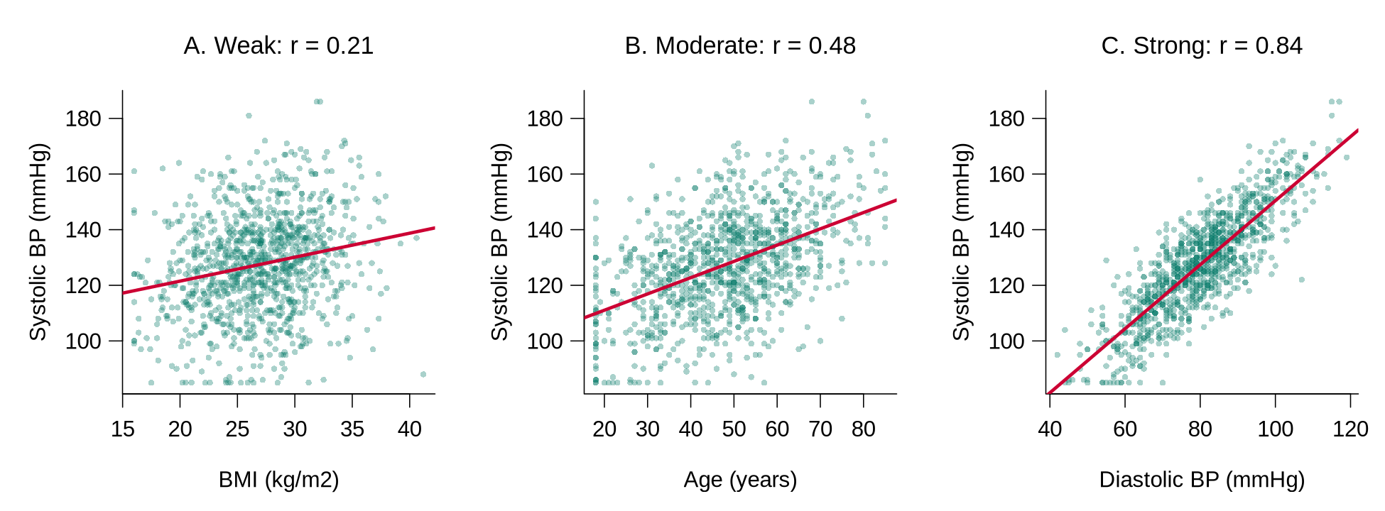
Worked Example 1.13 covers the middle row, a continuous outcome compared across groups, first for two groups and then for three. Notice that the regression coefficient for smokers equals the difference between the two group means.
Worked Example 1.13: One continuous and one categorical variable (systolic pressure by group)
For two groups, the group means and a simple linear regression answer the question together. tapply(x, group, mean) applies mean() to x separately within each group.
For three or more groups, one-way ANOVA tests whether the group means differ. The example uses the three age bands created earlier.
Reading the output. Mean systolic pressure is 126.3 mmHg among the 811 non-smokers and 131.5 mmHg among the 236 smokers. In the regression, the intercept (126.3) is the mean for the reference group, non-smokers, because No is the first level of smoker, and the coefficient smokerYes (5.15) is the difference between the two group means, with a 95% CI of 2.57 to 7.73 mmHg that excludes zero. In the ANOVA table, Df gives the degrees of freedom (number of groups minus 1, and number of people minus number of groups), Sum Sq and Mean Sq measure the variation between and within the groups, F value is the ratio of between-group to within-group variation, and Pr(>F) is the p-value. An F of 111.4 with p < 2e-16 indicates that mean systolic pressure differs across the age bands; ANOVA does not identify which bands differ, so the group means (115.6, 126.8, and 136.8 mmHg) are reported alongside it.
A model reporting sentence. “Mean systolic pressure was 131.5 mmHg among smokers and 126.3 mmHg among non-smokers, an unadjusted difference of 5.1 mmHg (95% CI 2.6 to 7.7). Mean systolic pressure also differed across age bands (one-way ANOVA, F = 111.4 on 2 and 1044 degrees of freedom, p < 0.001), rising from 115.6 mmHg in participants aged 35 or younger to 136.8 mmHg in those older than 55.”
Worked Example 1.14 covers the last row, two categorical variables. Check the expected counts as well as the p-value, because they decide whether the chi-squared test can be used.
Worked Example 1.14: Two categorical variables (smoking and hypertension)
A cross-tabulation counts the participants in every combination of two categorical variables, and row percentages make the groups comparable. prop.table(tab, margin = 1) divides each count by its row total.
The chi-squared test asks whether the pattern of counts differs from what would be expected if the two variables were unrelated. The expected count for a cell is the number of people who would fall in it if smoking made no difference to hypertension. By this we mean that the overall percentage with hypertension is applied to smokers and non-smokers alike, so each group is given the same share of hypertensive participants. The test then adds up how far each observed count lies from its expected count; the further apart they are, the larger the chi-squared statistic and the smaller the p-value. The expected counts are worth printing, because the test relies on an approximation that becomes unreliable when any expected count is small.
Reading the output. Hypertension is more common among smokers (35.2%, 83 of 236) than among non-smokers (28.4%, 230 of 811). The chi-squared statistic is 3.73 on 1 degree of freedom with p = 0.054. R applies a small correction (Yates’ continuity correction) automatically for a table with two rows and two columns. A p-value of 0.054 indicates weak evidence against no association: the data are somewhat unusual under no association, and a difference at least this large would arise in about 5 of every 100 samples of this size if there were no association. The crude difference will also change once age, a likely confounder, is taken into account. All expected counts are far above 5, so the test is appropriate here; when any expected count falls below 5, Fisher’s exact test, fisher.test(tab), is used instead.
A model reporting sentence. “Hypertension was more common among smokers (35.2%) than among non-smokers (28.4%), although the evidence for an unadjusted association was weak (chi-squared test, p = 0.054).”
All three examples report crude estimates, labelled as unadjusted, because nothing else is held constant. Their value lies in what they reveal before the multivariable model is planned.
7.4.2 What the Unconditional Associations Show
When evaluating unconditional associations, pay attention to three kinds of association:
- Associations between predictors and outcome: Determine if there is any association at all; determine the functional form (is it linear?); get a simple picture of the strength and direction. The functional form is the shape of the relationship. By this we mean whether the outcome changes by the same amount across the whole range of the predictor, as a straight line implies, or whether the relationship curves, levels off or changes direction. For example, a scatterplot may show that an outcome rises steeply at older ages but barely changes among younger adults, which would call for a squared term or a categorised version of the predictor in the later model.
- Associations between pairs of predictors: Look for potential collinearity problems (highly correlated predictors). Collinearity means that two predictors move together so closely that they carry much the same information. When both are placed in the same model, the model has great difficulty separating the effect of one from the effect of the other, and as a result their coefficients become unstable and their standard errors large. For example, systolic and diastolic pressure are strongly correlated, so a model that includes both as predictors may give an uncertain estimate for each.
- Confounding variables: Evaluate associations between the confounders identified in the causal diagram and the key predictors of interest and the outcome. These associations show how strongly each confounder could distort the crude comparison; the decision to adjust for a confounder rests on the diagram.
Collinearity between predictors is checked for all the continuous variables at once. Worked Example 1.15 does this with a correlation matrix; look for any pair whose correlation crosses the rule-of-thumb threshold.
Worked Example 1.15: Checking predictors for collinearity with a correlation matrix
A correlation matrix shows the correlation between every pair of continuous variables at once. cor() applied to several columns returns the matrix, and round(..., 2) keeps two decimal places.
Reading the output. Each cell is the correlation between the row variable and the column variable, and the diagonal is always 1. A common rule of thumb flags pairs with |r| above about 0.8 as possible collinearity problems. Systolic and diastolic pressure (r = 0.84) cross that line, which is expected because both measure blood pressure; a model would normally include one of them, or a combined measure, as a predictor. The correlation matrix helps detect collinearity, whereas the choice of confounders to include in a model comes from the causal diagram.
The unconditional analyses feed directly into the plan for the multivariable model. Table 1.12 lists common findings from these analyses and the next step each one calls for.
Table 1.12. Findings from the unconditional analyses and the next step each one calls for in planning the multivariable model.
| Finding | What to do next |
|---|---|
| A confounder from the DAG shows little crude association with the outcome. | The confounder stays in the planned model, because the decision to adjust rests on the causal diagram. |
| A scatterplot shows a curve. | The analyst plans a squared term (such as age_ctsq) or a categorised version (such as age_c3) for that predictor. |
| Two predictors have |r| above about 0.8. | The analyst treats them as candidates for collinearity and keeps the one that best matches the research question, or combines them. |
| A cross-tabulation has an expected count below 5. | The analyst uses Fisher’s exact test or combines sparse categories before modelling. |
| An association is far stronger or weaker than subject-matter knowledge suggests. | The analyst rechecks the coding and verification of both variables before interpreting it. |
Activity 1.4 runs the code of Worked Examples 1.7 to 1.15 on the blood pressure data in one narrated walkthrough, with three questions in the form used on the midterm. Run it along with the reading, then answer the questions from your own output.
Text version of the activity: the code of the run-along script, its console output and notes on reading it.
library(dplyr)
library(tidyr)
bp_raw <- read.csv("https://heal-learn.ca/r-activities/data/bp01.csv")   # course data, read from the website
bp_clean <- bp_raw |>
  drop_na(systolic, diastolic, age) |>
  mutate(age_c3 = cut(age, c(0, 35, 55, Inf), labels = c("young", "middle", "older")),
         htn = factor(systolic >= 140 | diastolic >= 90, levels = c(FALSE, TRUE),
                      labels = c("normotensive", "hypertensive")))
c(raw = nrow(bp_raw), clean = nrow(bp_clean))The raw file has 1092 participants, and the cleaned file keeps the 1047 with age, systolic and diastolic pressure recorded. It adds the three age bands age_c3 and the hypertension indicator htn (140/90 rule), as the recoding pipeline in Part 6 of Activity 1.2 does.
visits_a <- c(0, 2, 4, 3, 2, 6, 1, 3, 2, 3)    # clinic visits in a year, clinic A
visits_b <- c(0, 1, 1, 0, 9, 2, 0, 12, 1, 0)   # clinic visits in a year, clinic B
c(mean = mean(visits_a), var = var(visits_a))
c(mean = mean(visits_b), var = var(visits_b))
set.seed(4104)
los <- round(rlnorm(1000, meanlog = 1.2, sdlog = 0.8), 1)   # simulated length of stay (days)
summary(los)                     # before the log transformation
summary(log(los))                # after it
par(mfrow = c(1, 2)); hist(los, breaks = 40); hist(log(los), breaks = 30)Reading the output. Both clinics average 2.6 visits. In clinic A the variance (2.71) is close to the mean, as a Poisson model expects; in clinic B it is 18.27, far larger than the mean, which is overdispersion, so negative binomial regression is the safer starting point. For the simulated length of stay, the mean (4.57 days) is well above the median (3.40 days), a numerical sign of right skew; after log() the mean (1.19) and median (1.22) are close and the histogram is roughly symmetric. The logarithm is defined only above zero, so an outcome with zeros needs adjustment first, for example log(x + 1).
colSums(is.na(bp_raw))                         # number missing per variable
round(100 * colMeans(is.na(bp_raw)), 1)        # percentage missing per variable
bp_clean <- bp_clean |>
  mutate(age_dec = cut(age, c(17, 29, 39, 49, 59, 69, 79, Inf),
                       labels = c("18-29", "30-39", "40-49", "50-59", "60-69", "70-79", "80+")))
table(bp_clean$age_dec, bp_clean$htn)
bp_clean <- bp_clean |>
  mutate(age_dec6 = cut(age, c(17, 29, 39, 49, 59, 69, Inf),
                        labels = c("18-29", "30-39", "40-49", "50-59", "60-69", "70+")))
table(bp_clean$age_dec6, bp_clean$htn)Reading the output. Age is missing for 11 participants (1.0%), systolic pressure for 18 (1.6%) and diastolic pressure for 19 (1.7%); because some participants miss more than one, the cleaned file (line 15) keeps 1047 of the 1092 participants. In the ten-year bands, 80+ has only 3 normotensive participants (and 14 hypertensive), so a logistic model would estimate that band from 3 people (odds ratio about 11 against 50 to 59, 95% CI from about 3 to more than 38). Merging 70 to 79 and 80+ into 70+ gives 24 normotensive and 49 hypertensive participants. Each decision is recorded in the analysis log with its numbers and its reason.
bp_long <- tribble(
  ~centre, ~person, ~visit, ~sbp,
  "A", "A01", 1, 132,   "A", "A01", 2, 128,   "A", "A02", 1, 141,
  "A", "A02", 2, 139,   "A", "A02", 3, 137,   "B", "B01", 1, 118,
  "B", "B01", 2, 121,   "B", "B02", 1, 150,   "B", "B03", 1, 126,
  "B", "B03", 2, 124)
count(bp_long, centre, person)                          # measurements per person
bp_long |> distinct(centre, person) |> count(centre)    # people per centre
n_distinct(bp_long$person) # people overallReading the output. People have between one and three measurements, centre A has two people and centre B three, and there are five people in all. Every identifier begins with the centre letter, so each person is uniquely identified across centres; otherwise a unique identifier is built first, for example with mutate(uid = paste(centre, person)). Observations from the same person or centre resemble one another, so a model that ignores the clustering gives standard errors that are too small.
cor.test(bp_clean$age, bp_clean$systolic)               # two continuous variables
plot(systolic ~ age, data = bp_clean)                   # scatterplot
fit1 <- lm(systolic ~ age, data = bp_clean)
cbind(estimate = coef(fit1), confint(fit1))
tapply(bp_clean$systolic, bp_clean$smoker, mean)        # continuous by two groups
fit2 <- lm(systolic ~ smoker, data = bp_clean)
cbind(estimate = coef(fit2), confint(fit2))
tapply(bp_clean$systolic, bp_clean$age_c3, mean)        # three or more groups
summary(aov(systolic ~ age_c3, data = bp_clean))
tab <- table(smoker = bp_clean$smoker, htn = bp_clean$htn)   # two categorical
tab
round(100 * prop.table(tab, margin = 1), 1)              # row percentages
chisq.test(tab)
chisq.test(tab)$expected # expected counts if unrelatedReading the output. Age and systolic pressure: r = 0.48 (95% CI 0.43 to 0.52), a moderate correlation, and a slope of 0.59 mmHg per year of age (95% CI 0.52 to 0.65). Smoking: mean systolic pressure 131.5 mmHg in smokers against 126.3 mmHg in non-smokers, a difference of 5.15 mmHg (95% CI 2.57 to 7.73). Age bands: means 115.6, 126.8 and 136.8 mmHg, F = 111.4 on 2 and 1044 degrees of freedom, p < 2e-16. Smoking and hypertension: 35.2% against 28.4%, chi-squared 3.73 on 1 degree of freedom, p = 0.054, with every expected count far above 5 (otherwise fisher.test(tab)). All of these are unadjusted. Question 3 adds round(cor(bp_clean[, c("age", "bmi", "systolic", "diastolic")]), 2), the correlation matrix used to check pairs of predictors for collinearity.
R Reflect on what you just ran
Answer each question from your own output, as on the midterm: justify each choice with evidence from the output, decide what to do about each problem and write the rule you would record in the analysis log, and say whether a variable should stay in the model and why.
1. For each of the three outcomes in part 2 of the script (clinic visits at clinic A, clinic visits at clinic B and hospital length of stay), state the model or processing step you would choose, and justify each choice with evidence from the output. Then state in one sentence what the log transformation did to the shape of the length-of-stay distribution.
log(los) instead. After the log transformation the mean (1.19) and the median (1.22) are close and the histogram is roughly symmetric, so the logarithm pulled in the long right tail; the new variable is created in the cleaning script and recorded in the codebook, and the residuals are still checked after the model is fitted.2. The output of lines 29 to 38 reveals two problems in the predictors: one in the missing-value counts and one in the cross-tabulation by ten-year age band. Identify the two problems, state for each whether you would keep, combine or exclude the affected values, and write the entry you would record in the analysis log.
3. Run your own code: at the end of your script, type and run round(cor(bp_clean[, c("age", "bmi", "systolic", "diastolic")]), 2), then tapply(bp_clean$age, bp_clean$smoker, mean), then coef(lm(systolic ~ smoker + age, data = bp_clean)). (a) Identify the problem the correlation matrix reveals for a model that would include these variables as predictors, and state what you would do about it. (b) The causal diagram in Worked Example 1.1 names age as a confounder of the effect of smoking. A colleague notes that smokers and non-smokers differ in mean age by only about two years and proposes to leave age out of the model. Based on these results and the theory driving the analysis, should age be removed? Why or why not?
tapply() shows that smokers are younger on average (46.3 against 48.6 years), and systolic pressure is about 0.59 mmHg higher per year of age, so leaving age out keeps the back-door path through age open and biases the smoking comparison. Adjusting for age moves the smoking difference from 5.15 mmHg (crude) to 6.48 mmHg, so the crude estimate understated it; the results table shows both, with the crude one labelled as unadjusted.Your output from Activity 1.4 takes the blood pressure data from processed variables to the crude associations that the multivariable model will build on, with each decision recorded in the log. The key takeaways below draw the section together before its knowledge check.
Key Takeaways
- 5.5 Before the serious modelling begins, set up a system for keeping track of what you run, because you will need to reconstruct every result and decision later. Work in blocks (all the single-variable summaries, then the two-variable associations, then the models), keep log files named after the scripts that produced them (for example, a Quarto or R Markdown report, or output saved with
sink()), and label and date every output. Record each decision with its reason, as the analysis-log entry in Worked Example 1.9 does for the complete-case decision and the 45 participants it excluded. A good test is whether you, three months from now, could trace any number in your report back to the script, the file version and the decision that produced it. - 7.1 Before modelling, check that each outcome suits the analysis you have planned, because the type of outcome sets the type of model. For a categorical outcome, check the count in each category and combine categories that hold only a handful of people, for example before a multinomial model. For a continuous outcome planned for linear regression, look at a histogram, and if it is strongly skewed, try a transformation such as the logarithm (
log()); a mean well above the median is a quick numerical clue to right skew, and the residuals are checked later, after the model is fitted. For a count, compare the mean with the variance usingmean()andvar(): when the variance is well above the mean (overdispersion, as in clinic B of Worked Example 1.7), negative binomial regression is a safer starting point than Poisson regression. - 7.2 Predictors get the same careful review, one at a time. First count the missing values, for example with
colSums(is.na()); if a predictor has many, you can drop it, run two analyses (one on the subset where it is present and one on the full dataset without it), or use multiple imputation, and whichever you choose goes in the analysis log with its reason. Then check that a continuous predictor is reasonably spread across its range (if it is not, it may need to be categorised) and that every category of a categorical predictor holds enough people, combining sparse categories, as the 70–79 and 80+ age bands were combined in Worked Example 1.10, so that estimates are stable. Scaling and recoding steps, such as centring age to makeage_ct, are made in the cleaning script and recorded in the codebook. A common trap is to drop a predictor, or fill its missing values with the mean, without saying so: a documented choice is defensible, and a silent one is not. - 7.3 Some datasets have a multilevel structure, with observations grouped inside larger units, such as repeated blood pressure measurements within people, or people within centres. Before modelling, find the average and range of the number of observations per higher-level unit (with
count()andn_distinct(), as in Worked Example 1.11) and make sure every individual has a unique identifier; if two centres both number their patients 01, 02, 03, build one first, for example withmutate(uid = paste(centre, person)). This matters because observations from the same person or centre resemble each other, so a model that ignores the clustering behaves as if it holds more independent information than it does, and its standard errors come out too small and its confidence intervals too narrow. Mixed models are built for this structure. In a question, clues such as repeated visits, several clinics, or one identifier appearing on several rows tell you that the data are multilevel. - 7.4 Before any multivariable model, look at the unconditional (crude) associations, one predictor at a time with nothing else held constant. The method depends on the two variable types: for two continuous variables, a scatterplot, a correlation coefficient (
cor()orcor.test()) and a simple linear regression; for one continuous and one categorical variable, group means with a one-way ANOVA (aov()) or a simple regression, or a simple logistic regression when the categorical variable is a binary outcome; and for two categorical variables, a cross-tabulation with row percentages and a chi-squared test (chisq.test()), with Fisher’s exact test when an expected count is below 5. These first looks show whether each association exists, its direction and rough strength, and whether it is straight or curved; a correlation matrix flags pairs of predictors with |r| above about 0.8 as possible collinearity; and the associations of each confounder with the exposure and the outcome show how much it could distort the crude comparison. A common trap is to drop a confounder from the DAG because its crude association is weak, when the decision to adjust rests on the diagram, not on the unconditional result. When you report one of these results, give the estimate with its 95% confidence interval and say that it is unadjusted, as in “each additional year of age was associated with a 0.59 mmHg higher systolic pressure (95% CI 0.52 to 0.65), before adjustment for other variables”.
1. An analyst plans a Poisson regression for the number of emergency department visits in a year. For a pilot sample of eight patients, the processing check gives the output below. What does it show?
> ed_visits <- c(0, 1, 0, 2, 0, 9, 1, 3)
> mean(ed_visits)
[1] 2
> var(ed_visits)
[1] 9.142857
> var(ed_visits) / mean(ed_visits)
[1] 4.571429
2. A logistic regression of diabetes (yes or no) on education is planned. The cross-tabulation of the predictor with the outcome is shown below. What should be done before the model is fitted?
| Education | No diabetes | Diabetes |
|---|---|---|
| Less than high school | 9 | 2 |
| High school | 210 | 41 |
| College | 388 | 52 |
| University | 301 | 27 |
3. A file holds three HbA1c measurements for each of 400 patients, and the patients attend 12 clinics, so the file has 1,200 rows. A colleague proposes to analyse the rows as 1,200 independent observations. What is the likely consequence, and what should be checked first?
count() and n_distinct() (here 3 measurements per patient, and the number of patients in each of the 12 clinics) and makes sure that no two patients share an identifier. Option (c) is tempting because more rows usually mean more power, but that apparent extra power is exactly the false precision the clustering creates, and option (b) reverses the direction of the error. (Section 4, slide “Characterise the hierarchy before modelling”, 7.3 Recognising Multilevel Data and Worked Example 1.11; Objective 7.3)4. Before fitting a multivariable model, an analyst wants the unconditional association for each of three pairs: (i) BMI (kg/m²) and systolic pressure (mmHg); (ii) systolic pressure across three income groups; and (iii) smoking (yes or no) and hypertension (yes or no). Which set of methods matches the variable types?
5. During the unconditional analyses, an analyst merges the two oldest age bands into one and decides on a complete-case analysis for income, which is missing for 36 of 1,200 participants. Which record of these decisions meets the standard for keeping track of analyses?
6. A school health team will model the number of school days missed by 600 students, with asthma as the exposure and household income and household smoking as confounders in the causal diagram. The missing-value check is shown below. A colleague suggests dropping income from the analysis and not mentioning it in the report. Which response follows the lesson?
> colSums(is.na(sch))
days_missed      asthma      income    hh_smoke
          0           0         162           0
> round(100 * colMeans(is.na(sch)), 1)
days_missed      asthma      income    hh_smoke
          0           0          27           0
> sum(!is.na(sch$income))
[1] 438
A Structured Approach to Data Analysis: Final Assessment
Bringing It All Together
This lesson laid out a structured workflow for taking a dataset from collection to first analysis. The first section insisted that you start with a causal diagram and a clear separation of outcomes, predictors, confounders, and intervening variables, before you touch the data. The section on coding, entry, and file management turned that intent into discipline at the level of files: thoughtful coding, a project folder you could hand to a collaborator, and a codebook that captures every variable. The section on program files and verification made the workflow reproducible by moving you out of point-and-click interactive mode into program-mode scripts, with systematic editing and verification. The section on data processing closed the loop by processing outcomes and predictors, surfacing multilevel structure, and producing the unconditional associations that should always precede a multivariable model.
The thread running through all four sections is that an analysis is only as trustworthy as the steps that came before it. Every modelling method, including linear regression, model building, logistic regression, count models, and mixed models, assumes you arrive at the modelling step with a clean, documented, and well-understood dataset. The structured approach is what makes that modelling possible. It also positions you to interpret p-values, confidence intervals, and effect sizes responsibly when you eventually report them (Wasserstein & Lazar, 2016; Greenland et al., 2016), and to avoid the analytic flexibility that drives false-positive results (Simmons, Nelson, & Simonsohn, 2011). A first plain-language reading of a p-value and a confidence interval accompanies the mediation example in the first section, and the worked examples of unconditional associations apply both; the same two quantities are reported with every model. The historical roots of exploratory data analysis trace to John Tukey.
Key Takeaways from this lesson
- You can now explain why a trustworthy analysis follows a structured, iterative workflow: causal diagram, cleaning and verification, unconditional checks, and only then the multivariable model, with every step run from a saved script in program mode. Backing up several steps as you learn about the data is normal, and the script is the honest record that lets anyone rerun what you did. When an exam plan jumps straight to a model, lets p-values choose the variables, or relies on unsaved point-and-click steps, name the step that was skipped and explain what could go wrong as a result.
- You can read a causal diagram and name the outcome, the exposure, and any confounders (forks), mediators or intervening variables (chains) and colliders, using only the direction of the arrows. The most useful habit is to trace the arrows for every variable one at a time and to say so when a role is absent: “no mediator” can be the right answer, a variable that only causes the outcome is not a confounder, and an arrow pointing at another arrow marks a moderator.
- You can read the adjustment set from a diagram (confounders in, mediators out when the total effect is wanted, colliders never) and explain what each wrong decision costs: confounding bias, a direct effect in place of the total effect, or a false association created by adjusting for or selecting on a collider. In an exam answer, state the model in one sentence, then give the reason and the consequence of the wrong choice for each variable in turn.
- You can read a raw file against its data dictionary and find the common coding faults: a missing code that could be a real value, text in a numeric field, a compound code, mixed date formats and mixed missing-value conventions. For each one, name the fault and its best-practice correction, and remember that every correction is made in the cleaning script, never by editing the raw file by hand.
- You can describe a system that protects the original data and leaves an audit trail: originals kept and checked early for completeness, double data entry with a programmed comparison, raw data kept read-only, versioned file names that are never overwritten, a file log, systematic variable names with a codebook, and a log of analyses run in blocks. The practical test for any part of the system is whether someone else could trace every number back to the original form, the file version and the decision that produced it.
- You can describe the scripted editing (variable labels, category labels and every missing code converted to
NA) and the verification checks (valid and missing counts, smallest and largest values, histograms, frequency tables and cross-variable checks) made before analysis, and you can use their output to spot implausible values and unexpected categories. When you readsummary()ortable()output, compare every minimum, maximum and category with what is possible and with what the codebook allows. - You can process outcome and predictor variables for the planned model, recognise multilevel structure, choose the unconditional analysis for each pair of variable types, and explain what those first analyses reveal about functional form, collinearity and confounders. Keep the matching in mind: two continuous variables call for a correlation, scatterplot and simple regression, one continuous and one categorical variable for group means with ANOVA or a simple regression, and two categorical variables for a cross-tabulation with a chi-squared test. Remember too that a weak crude association never removes a confounder from the model, because that decision rests on the diagram.
Final Knowledge Assessment
1. A colleague says: “Drawing a causal diagram before we look at the data is a formality. We can enter every variable, keep the ones with p < 0.05, and let the model tell us what matters.” Which reply best explains why the lesson puts the causal diagram first?
2. A student counts the students with and without asthma in each age group in a spreadsheet, types those counts into the R Console to run a chi-squared test, and saves only the final printed result. Which critique follows the lesson?
3. A campus health team asks whether food insecurity (the exposure) increases depressive symptoms (the outcome) among university students. Its causal diagram (below) has these arrows: household income → food insecurity, household income → depressive symptoms, food insecurity → poor sleep → depressive symptoms, food insecurity → depressive symptoms, food insecurity → wellness-centre visits ← depressive symptoms, and an arrow from international student status that ends on the arrow from food insecurity to depressive symptoms. Which classification is correct?
4. In the diagram in Question 3, the arrow from international student status ends on the middle of the arrow from food insecurity to depressive symptoms, rather than on either variable. How should international student status be classified?
5. A study asks whether neighbourhood green space (the exposure) reduces childhood asthma (the outcome). Its causal diagram (below) has these arrows: green space → asthma, green space → physical activity → asthma, air pollution → asthma, and green space → survey participation ← asthma. Which statement about the diagram, as drawn, is correct?
6. For the diagram in Question 3 (household income → food insecurity and household income → depressive symptoms; food insecurity → poor sleep → depressive symptoms; food insecurity → wellness-centre visits ← depressive symptoms; international student status pointing at the arrow from food insecurity to depressive symptoms), which variables must be adjusted for to estimate the total effect of food insecurity on depressive symptoms?
7. Using the diagram in Question 3, a model of the depressive symptom score (0 to 27 points) on food insecurity, adjusted for household income, gives a food-insecurity coefficient of 3.2 points. A colleague then adds poor sleep to the model “to be safe”, and the coefficient falls to 1.9 points. Which interpretation is correct?
8. The first three rows of a raw smoking-cessation file are shown below; the data dictionary describes visit_date as “date of clinic visit” and cigs_day as “cigarettes smoked per day”. Which pair of faults and corrections is correct?
id    visit_date   cigs_day
K01   2024-11-02   12
K02   02/11/2024   ten
K03   3 Nov 24     0
cigs_day column into text, so R cannot calculate with it, and the number the word means is recorded instead. Option (d) is tempting because it chooses one format, but DD/MM/YYYY is itself the ambiguous form, and it leaves the text in place; the 0 in option (c) is the real answer of a participant who does not smoke and must not become missing. (Section 2, 4.1.2 Spotting Coding Faults in a Raw File; Objective 4.1)9. A perinatal file records bwt_g, birth weight in grams, and its data dictionary states “999 = not recorded”. The file includes infants born very preterm, some of whom weigh less than 1,000 g at birth. What is the fault, and how should it be corrected?
NA in the script. Option (d) is tempting because the code is documented, but documentation cannot tell a real 999 g infant from a missing record; option (a) mistakes an unusual value for an impossible one. (Section 2, slide “Three rules that prevent cascading errors”, 4.1.2 Spotting Coding Faults in a Raw File and Worked Example 1.4; Objective 4.1)10. Four entries from a draft data dictionary are listed below. Which entry follows the coding rules taught in this lesson?
11. A research coordinator proposes four practices for a new influenza study. Which one would put the data at risk and break the audit trail?
12. An adult nutrition survey records weight_kg. The verification check of the extreme values gives the output below. Which values should be investigated?
> head(sort(dat$weight_kg), 5)
[1]  0.0 38.2 41.5 43.0 44.8
> tail(sort(dat$weight_kg), 5)
[1] 131.0 136.4 142.9 680.0 999.0
NA if it is a missing code), and the check is repeated, because where there is one error there are often more. Option (a) is tempting because 999 is the familiar code, but 0.0 and 680.0 are just as impossible; option (c) misreads the purpose of the check, which is to inspect the extremes, not to delete them. (Section 3, slide “Check before you trust”, 6.2 Verifying the Data and Table 1.8; Objective 6.2)13. The codebook allows three values for vacc_status: Complete, Partial and None. The first frequency table is shown below. What should the cleaning script do?
> table(dat$vacc_status, useNA = "ifany")

complete Complete     none     None  Partial     <NA>
       6      412        3       58      133       11
NA; the rerun table then lists only the codebook categories. Option (d) is tempting because it removes the unexpected categories, but it throws away answers whose meaning is clear and adds to the missing values; option (b) also edits the raw file by hand. (Section 3, slide “Three components of scripted editing”, 6.2 Verifying the Data and “Reading the fix in Activity 1.3”; Objective 6.2)14. Before fitting a model for the effect of physical activity on systolic pressure, the unconditional analyses show that BMI and waist circumference are highly correlated (r = 0.88), and that age, a confounder in the causal diagram, has only a weak crude association with systolic pressure (r = 0.08). Which plan follows from these findings?
15. The planned outcome for a linear regression is the cost of a hospital stay, in dollars, for 900 patients. Its summary is shown below. What does the processing step suggest?
> summary(dat$cost)
   Min. 1st Qu.  Median    Mean 3rd Qu.    Max.
     90     900    2020    3361    3982   43780
16. A regional health authority gives you walk01.csv, the raw file of a survey of 1,800 adults aged 50 and over, to study whether owning a dog (the exposure) is associated with weekly minutes of walking (the outcome). A colleague proposes to correct odd-looking values by typing over them in a spreadsheet and saving the file under the same name, and then to enter all 40 variables, including the number of dog walks per day, into one model and keep those with p < 0.05. Which revised plan follows the structured approach of this lesson?
✦ Before submitting: pass every section knowledge check (100%).